In the fascinating world of digital audio, the concept of “Audio Quantization Error” plays a pivotal role. Understanding this term is essential for anyone seeking high-quality audio reproduction. Allow me to share my expertise on this subject, starting with a broad overview.
Demystifying Audio Quantization Error
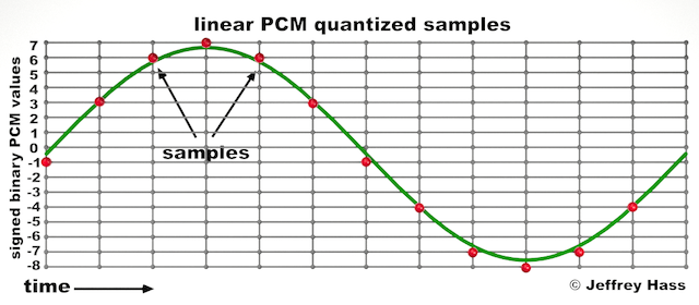
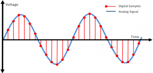
Audio quantization error is a fundamental aspect of digital audio processing. When analog sound waves are converted into digital signals, they undergo quantization. This means that the continuous analog signal is sampled and approximated in discrete steps. These steps are represented by binary values, typically in the form of bits (e.g., 16-bit, 24-bit). Now, what’s crucial to grasp here is that these discrete steps can lead to imperfections in audio reproduction.
Quantization error, often referred to as “quantization noise,” occurs when the actual analog signal deviates from the approximated digital representation. Imagine you have a beautiful painting, and you’re asked to replicate it using only a limited set of colors. The more restricted your color palette, the less accurate your reproduction will be. In the same way, the fewer bits you use for audio quantization, the more pronounced the quantization error becomes.
Quantization Levels and the Impact on Sound Quality
The number of quantization levels (related to bit depth) directly affects the precision of audio representation. For instance, a 16-bit audio recording has 65,536 possible levels, while a 24-bit recording provides a staggering 16,777,216 levels. This increased bit depth allows for a much finer representation of the original analog signal. Hence, a higher bit depth results in a reduction of quantization error, leading to superior sound quality.
To illustrate this, consider a grayscale image with only two colors: black and white. This is akin to an extremely low bit depth in audio, where the audio signal is either “on” or “off.” Now, imagine a high-resolution image with millions of colors, similar to the detail you get in a 24-bit audio recording. The difference in quality is apparent.
The Role of Dithering in Minimizing Quantization Error
One might wonder if there’s a way to mitigate quantization error in low-bit-depth audio recordings. Enter “dithering.” Dithering is a technique that introduces low-level noise to the audio signal, effectively spreading out the quantization error across a broader spectrum. Think of it as adding a sprinkle of fine grains of sand to a painting to blend the colors. This subtle noise masks the harshness of quantization error and makes it less noticeable to the human ear.
Now, as we’ve explored the fundamentals of audio quantization error, let’s delve into the questions that often arise:
How Does Quantization Error Affect Music Production?
In the realm of music production, quantization error can be a significant concern, particularly for professionals aiming to achieve top-tier sound quality. When producing music, especially in genres where subtle nuances are crucial, such as classical or jazz, quantization errors become more perceptible. To maintain audio fidelity, a higher bit depth is preferred during recording and production, ensuring minimal quantization noise.
Is There an Ideal Bit Depth for Audio Recording?
The ideal bit depth for audio recording is a subject of debate among audio enthusiasts. While 24-bit recording is commonly favored for its excellent dynamic range and low quantization error, it’s worth noting that the final audio format for most consumer applications, like CDs or streaming, is often 16-bit. The choice of bit depth should be based on the specific requirements of the project, keeping in mind the trade-off between audio quality and file size.
Can Quantization Error be Completely Eliminated?
Regrettably, quantization error cannot be entirely eliminated, as it’s an inherent part of the digital audio conversion process. However, it can be minimized to the point where it’s imperceptible to the human ear. Through techniques like dithering and the use of higher bit depths, the impact of quantization error can be significantly reduced, allowing for exceptional audio quality.
Last Words about Audio Quantization Error
In the ever-evolving world of audio technology, understanding audio quantization error is a fundamental step towards achieving superior sound quality. As an expert in the field, I’ve shared insights, experiences, and technical knowledge to demystify this concept. Remember, the bit depth you choose in audio recording significantly influences the extent of quantization error, and techniques like dithering play a pivotal role in mitigating its effects. The quest for pristine audio quality is an ongoing journey, but armed with this knowledge, you’re better equipped to make informed decisions in your audio endeavors.
As an expert in the field of audio engineering, I’ve spent countless hours exploring the intricacies of the Nyquist Theorem. This foundational concept is the bedrock of modern digital audio processing, and its significance cannot be overstated. The Nyquist Theorem, in essence, defines the minimum sampling rate required to accurately convert analog signals into digital form.
Think of it this way: imagine you’re watching a fast-moving train and trying to take photographs to capture its motion. If you snap pictures too infrequently, you won’t capture the train’s true movement; details will be lost. The Nyquist Theorem tells us that in audio, the sampling rate must be at least twice the highest frequency we wish to reproduce. It’s the key to ensuring that nothing is missed when we transform the analog world of sound into the digital realm.
Now, let’s explore this concept further. Imagine you’re at a live music concert, and the artist hits a soaring high note. If your recording equipment doesn’t sample at a rate higher than the Nyquist frequency for that note, you’ll hear distortion and unwanted artifacts. Understanding the Nyquist Theorem is essential for audio engineers and music producers, as it directly impacts the quality of the final product, allowing us to capture and reproduce sound faithfully.
Applying Nyquist in Audio Recording
When it comes to audio recording, applying the Nyquist Theorem is akin to wielding a precision instrument. It’s not just a theoretical concept; it’s a practical guide for achieving clarity and fidelity in recorded audio. Consider it the compass that ensures we’re on the right path when capturing analog sound in the digital realm.
Imagine you’re recording a vocal performance. The Nyquist Theorem guides you in selecting the appropriate sampling rate for your digital recorder. If you neglect this principle and sample at a rate lower than twice the highest frequency in the vocalist’s range, you risk introducing aliasing, a phenomenon where high-frequency components are erroneously mapped to lower frequencies. This results in a distorted, unnatural sound, akin to viewing a pixelated image.
By heeding the Nyquist Theorem, audio engineers and recording artists ensure that their work preserves the subtle nuances and dynamic range of sound, producing recordings that captivate and resonate with listeners.
The Significance of Nyquist Frequency
Within the realm of digital audio, the Nyquist frequency stands as a sentinel of sound quality. Picture it as a gatekeeper, defining the boundary between faithful reproduction and unwanted distortions. It plays a pivotal role in digital audio, similar to how a camera’s shutter speed determines the clarity of a photograph.
Let’s delve into this further: suppose you’re designing an audio system. To prevent aliasing, you must set the sampling rate based on the Nyquist frequency. This ensures that the system captures and reproduces sound accurately. It’s analogous to building a bridge with a weight limit to ensure safety. By acknowledging the Nyquist frequency’s significance, audio engineers create systems that consistently deliver high-quality sound experiences.
Whether you’re a musician, audio engineer, or simply an audio enthusiast, recognizing the importance of the Nyquist frequency empowers you to make informed choices about equipment, software, and recording techniques, ultimately elevating your sonic experiences.
High Sampling Rates and Audio Quality
The impact of high sampling rates on audio quality is profound and undeniable. It’s the difference between a breathtaking high-definition image and a blurry snapshot. In the audio world, a high sampling rate means capturing more snapshots per second, preserving the intricate details of the sound waveform.
Imagine you’re in a studio recording a delicate acoustic guitar performance. To capture the subtle harmonics and nuances, a high sampling rate is essential. It’s like using a magnifying glass to appreciate the intricate details in a work of art. Musicians and audio engineers often opt for higher sampling rates, as they enable the faithful reproduction of every note and texture, resulting in recordings that feel alive and immersive.
Investing in high-quality equipment that supports high sampling rates is a testament to your commitment to audio excellence. It’s the path to creating soundscapes that resonate with audiences and evoke emotions on a profound level.
Avoiding Aliasing in Digital Audio
Avoiding aliasing in digital audio is a crucial mission for any audio engineer or producer. Imagine aliasing as the unwelcome ghost that haunts your recordings, distorting the beauty of sound. It occurs when the Nyquist sampling rate is not observed, and higher frequencies masquerade as lower ones, resulting in unpleasant artifacts.
Think of aliasing as a mirror that distorts your reflection; it’s not an accurate representation of reality. To banish this ghost, you must adhere to the Nyquist Theorem’s principles diligently. Use filters and sample at rates that prevent high-frequency components from sneaking into lower frequencies.
By doing so, you ensure that your digital audio productions are clean, pure, and devoid of unwanted artifacts. It’s akin to restoring a classic painting, revealing its true beauty without distortion or blemishes.
Last Words
“In the world of audio, the Nyquist Theorem is our guiding star. It empowers us to capture the magic of sound faithfully. Whether you’re recording a symphony, crafting a podcast, or simply savoring your favorite music, understanding the Nyquist Theorem unlocks a world of sonic possibilities. Let it be your compass in the realm of audio excellence.” — William Kindall, Audio Expert
Digital Bit Depth in AudioDigital Bit Depth in Audio
Digital bit depth in audio is a fundamental concept that impacts the quality and fidelity of digital sound. Bit depth, also known as audio resolution, refers to the number of bits used to represent the amplitude of an audio signal at a specific point in time. It essentially quantifies how finely audio samples are taken in the digital domain.
To put it simply, the bit depth determines the precision with which sound is captured and stored digitally. Common bit depths in digital audio are 16-bit, 24-bit, and 32-bit, with higher numbers providing greater precision.
Audio Bit Depth Explained
Understanding audio bit depth is essential for anyone seeking to grasp the intricacies of digital audio recording and playback. At its core, audio bit depth is a measure of how accurately an analog sound wave’s amplitude is captured and converted into a digital signal.
In practical terms, a higher bit depth signifies that the digital representation of an audio waveform closely mirrors the original analog signal, resulting in reduced quantization error or “noise.” Quantization error occurs when an analog value is approximated to the nearest digital value, and lower bit depths can make this error more noticeable, especially in quieter sections of audio.
Bit Depth and Audio Quality
Bit depth plays a pivotal role in determining the quality and precision of digital audio. The relationship between bit depth and audio quality is akin to an artist’s palette of colors. A higher bit depth provides a broader spectrum of shades and nuances, making the digital representation of sound more faithful to the original analog source.
For example, a 16-bit system offers 65,536 discrete amplitude levels, whereas a 24-bit system provides an astonishing 16,777,216 levels. This heightened precision results in smoother and more detailed audio representation, particularly in the subtle and quiet passages of a recording.
Digital Audio Resolution
Digital audio resolution, closely linked to bit depth, is a critical factor in capturing and reproducing sound accurately. It refers to the level of detail and clarity in digital audio. The greater the bit depth, the higher the resolution, and the finer the nuances that can be captured.
In the realm of audio production, higher digital audio resolution means that the subtle nuances, such as the intricacies of a singer’s voice or the delicate harmonics of a musical instrument, are preserved with remarkable fidelity.
Bit Depth in Music Recording
In the world of music recording, selecting the appropriate bit depth is a crucial decision that profoundly affects the final audio quality. Musicians and producers carefully consider bit depth when recording to ensure that the nuances and dynamics of their performances are accurately captured.
In practice, 24-bit recording is a popular choice among music professionals. This bit depth provides an ideal balance between precision and file size, allowing for the capture of subtle details while minimizing the risk of bit-depth noise in quieter sections of the recording.
Audio Signal Precision
Audio signal precision, often measured by bit depth, is a key consideration in professional audio production. It relates to how faithfully an audio system can reproduce the original sound. The higher the bit depth, the greater the precision in representing the analog signal, resulting in cleaner and more accurate audio playback.
For audio engineers and producers, achieving optimal audio signal precision is paramount. It ensures that the music they create is heard as intended, with all the intricacies and subtleties faithfully reproduced.
Bit Depth in Analog-to-Digital Conversion
Understanding how bit depth influences analog-to-digital conversion is essential for maintaining audio fidelity. Analog-to-digital conversion is the process of transforming continuous analog signals into discrete digital values. Bit depth determines the number of discrete values that can represent the amplitude of the analog signal during this conversion.
In essence, higher bit depth means that the analog-to-digital conversion process captures more precise details from the analog signal. This is particularly critical when working with high-quality audio sources where preserving every nuance is paramount.
Sound Fidelity and Bit Depth
Sound fidelity, the faithfulness with which audio is reproduced, is intricately linked to bit depth. A higher bit depth generally results in better audio fidelity, as it allows for the accurate representation of both subtle nuances and powerful crescendos in music.
Consider classical music or jazz, where dynamics play a significant role. With a higher bit depth, the audio system can faithfully reproduce the full range of soft and loud passages, ensuring that the listener experiences the music as intended by the performers and composers.
Impact of Bit Depth on Audio Playback
The impact of bit depth on audio playback is a critical factor in delivering a high-quality listening experience. When you listen to digital audio, the bit depth of the source file significantly affects what you hear.
In simple terms, higher bit depth in the source audio file results in a more faithful and detailed listening experience. This becomes especially noticeable in acoustic instruments, where the subtle nuances of a violin’s bowing or a pianist’s touch can be lost in lower bit depth recordings.
How Does Bit Depth Affect the Quality of Digital Audio?
Exploring how bit depth affects the quality of digital audio is crucial for audiophiles and audio professionals alike. It’s the bit depth that determines how accurately the audio signal is captured and reproduced, ultimately influencing the overall audio quality.
A higher bit depth translates to a more faithful representation of the original sound, with fewer imperfections or noise introduced during the recording and playback processes. This improvement in audio quality is particularly noticeable in genres that require a wide dynamic range and high levels of detail.
What Is the Role of Bit Depth in Recording Music Digitally?
The role of bit depth in recording music digitally is a multifaceted aspect of audio production. When musicians and engineers step into the studio, they must make critical decisions about bit depth to ensure that their recordings capture the essence of the music.
Choosing the appropriate bit depth is a balancing act. While higher bit depths provide greater precision and fidelity, they also result in larger file sizes. Musicians often opt for 24-bit recordings as they strike a harmonious balance between capturing subtle details and managing storage requirements.
How Is Audio Fidelity Influenced by Digital Bit Depth?
Understanding how digital bit depth influences audio fidelity is key to achieving top-tier sound quality. Audio fidelity, often described as the faithfulness of audio reproduction to the original source, is a critical consideration for audio professionals and enthusiasts.
With a higher bit depth, audio fidelity is enhanced because the digital representation of the sound is more detailed and accurate. This is especially crucial in professional audio production, where maintaining the highest possible fidelity is paramount.
Can You Explain the Importance of Bit Depth in Analog-to-Digital Conversion for Audio?
Explaining the importance of bit depth in analog-to-digital conversion sheds light on the intricacies of audio processing. Analog-to-digital conversion is the bridge that allows analog sound to be translated into a digital format that can be manipulated and stored. Bit depth plays a pivotal role in this process.
Higher bit depths ensure that the analog-to-digital conversion process captures more fine-grained details from the original analog signal. This is essential for preserving the richness and subtleties of audio, whether it’s a soaring vocal performance, the resonance of a musical instrument, or the ambiance of a recording environment.
What Is the Relationship Between Bit Depth and Dynamic Range in Digital Audio?
The relationship between bit depth and dynamic range in digital audio is a crucial one to understand. Dynamic range refers to the difference between the softest and loudest sounds that an audio system can reproduce. Bit depth plays a pivotal role in defining this dynamic range.
Higher bit depths translate to a wider dynamic range, allowing for the faithful reproduction of both subtle nuances and powerful crescendos in music. This is essential for maintaining audio fidelity, especially in genres with a wide range of dynamics, such as classical music and jazz.
How Does Bit Depth Impact the Accuracy of Audio Playback?
The impact of bit depth on the accuracy of audio playback cannot be overstated. When you listen to music or any digital audio content, the bit depth of the source file has a profound influence on what you hear.
Higher bit depth in the source audio file means that the playback faithfully represents the original recording. It allows for the subtlest details and nuances to shine through, creating a more immersive and engaging listening experience. In essence, higher bit depth contributes to the accuracy and realism of audio playback.
Are There Industry Standards for Bit Depth in Digital Audio Recording?
In the world of professional audio recording, industry standards play a vital role in guiding the use of bit depth. While there’s flexibility in choosing bit depths based on specific requirements, certain standards are commonly followed.
For instance, most audio CDs use 16-bit resolution, which offers high-quality playback suitable for the majority of consumers. However, in the realm of studio recording and mastering, 24-bit and even 32-bit formats are commonly employed to ensure the highest level of fidelity.
What Are the Advantages of Using Higher Bit Depth in Audio Processing?
Using higher bit depth in audio processing offers several distinct advantages. These advantages extend to both recording and post-production stages, and they significantly impact the overall quality of audio content.
Enhanced Audio Fidelity
One of the primary advantages is enhanced audio fidelity. Higher bit depths provide more precision in capturing and reproducing audio, resulting in recordings that faithfully preserve the original sound. This is particularly important in professional music production and critical listening environments.
Greater Dynamic Range
Higher bit depths also grant a greater dynamic range, allowing for the faithful representation of a wide range of sound intensities. This is particularly beneficial in genres of music or audio content with stark differences in volume, as it ensures that both delicate subtleties and powerful peaks are accurately reproduced.
How Can I Optimize Bit Depth for Better Audio Resolution?
For those involved in audio production or seeking the best listening experience, optimizing bit depth is crucial. It’s not just about using the highest available bit depth but also considering the entire audio workflow and ensuring that bit depth aligns with specific needs.
Matching Bit Depth to Audio Source
When recording audio, it’s essential to match the bit depth to the dynamic range of the audio source. For instance, a live jazz performance with wide dynamic swings benefits from 24-bit recording, while a podcast with a more consistent volume may suffice with 16-bit. This approach minimizes bit-depth noise while preserving audio quality.
Post-Production Considerations
During post-production, maintaining a high bit depth throughout the editing and mixing process is advisable. Only when preparing the final distribution format, such as a CD or streaming file, should the audio be converted to a lower bit depth to match the destination format.
The Benefits of Greater Bit Depth in Digital Audio Systems
As technology advances, digital audio systems are offering higher bit depths as an option. But what are the practical advantages of embracing these extended bit depths?
Future-Proofing Audio
One significant advantage is future-proofing your audio recordings. With higher bit depths, your recordings are better equipped to stand the test of time. As playback systems and formats improve, your high-bit-depth recordings will continue to sound exceptional, ensuring that your music or audio content remains relevant for years to come.
Editing Flexibility
Greater bit depths also provide increased editing flexibility. Audio engineers can apply effects and processing without worrying as much about introducing quantization errors or compromising audio quality. This freedom allows for more creative experimentation during the mixing and mastering stages, ultimately leading to more polished and refined audio content.
In conclusion, digital bit depth is a critical factor in the world of audio, influencing both recording and playback quality. Understanding its importance, selecting the appropriate bit depth for various scenarios, and embracing higher bit depths when possible can lead to an audio experience that is richer, more immersive, and of the highest fidelity. Whether you’re a musician, audio engineer, or simply a music enthusiast, appreciating the role of bit depth can elevate your audio journey to new heights.
Digital audio is a method of storing audio data on a computer or digital device. Audio data is essentially a collection of sound waves, and to store it digitally, we need to convert these sound waves into a series of numbers that a computer can understand.
What is Digital Audio?
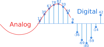
To do this, we use a process called “analog-to-digital conversion”. Analog audio signals are transformed into digital data by measuring the sound wave at regular intervals and assigning each measurement a numerical value. The process of measuring sound waves is called “sampling”, and the numerical values assigned to each sample are known as “bit depth”.
In essence, the audio signal is converted into a series of binary digits (1s and 0s) that can be stored on a computer. This allows us to manipulate, edit, and reproduce audio data in various ways.
How is Audio Converted to Digital Audio?
As mentioned earlier, audio is converted to digital audio using a process called “sampling”. Sampling involves taking snapshots of the audio signal at regular intervals, known as the “sampling rate”. The more samples that are taken per second, the more accurately the original sound can be reconstructed.
Imagine taking a picture of a person running. If you take one picture per second, you’ll see the person moving, but the motion won’t be smooth. If you take 10 pictures per second, the motion will be smoother, and if you take 60 pictures per second, the motion will be very smooth.
The same principle applies to digital audio. By taking many samples per second, the original sound can be accurately reconstructed. The number of samples taken per second is called the “sampling rate”, and it’s usually measured in Hertz (Hz). For example, a typical sampling rate for CD-quality audio is 44.1kHz, which means that 44,100 samples are taken per second.
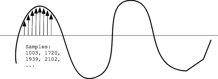
Once the audio has been sampled, each sample is converted into a digital number. The number represents the amplitude of the sound wave at that particular moment. The amplitude of a sound wave is the height of the wave, and it determines how loud or quiet the sound is.
The digital numbers obtained from each sample are stored as binary data, which can be easily stored, edited, and reproduced on a computer.
What is an MP3?
An MP3 is a type of digital audio file that uses a technique called “lossy compression”. This means that some of the data in the original audio file is removed in order to reduce the file size. The removed data is typically inaudible to the human ear, so the overall quality of the audio is not significantly affected.
MP3s achieve this compression by using a technique called “perceptual coding”. This involves analyzing the audio signal and identifying the parts that are less important to the overall sound quality. These parts are then removed, leaving only the most important parts of the audio signal intact.
For example, let’s say you have a song that is 4 minutes long and takes up 40MB of storage space on your computer. If you were to convert that song into an MP3 file, the resulting file might only be 4MB in size, while still maintaining a high level of audio quality.
MP3 files are a popular choice for digital audio because they take up less space than other audio formats, making them easier to store and share. They’re also supported by most digital audio players and software, making them a versatile and widely used format.
How are Sound Waves Converted into Digital Numbers?
As we mentioned earlier, sound waves are converted into digital numbers using a process called “analog-to-digital conversion”. This process involves several steps:
Sampling: The analog audio signal is measured at regular intervals, known as the sampling rate. Each sample is a snapshot of the audio signal at that particular moment.
Quantization: Each sample is assigned a numerical value that represents the amplitude of the sound wave at that moment. This is done using a process called quantization, which assigns a specific digital value to each sample.
Encoding: The digital values obtained from quantization are then converted into binary data. This is done using a process called encoding, which converts each digital value into a series of 1s and 0s.
Compression: Depending on the file format being used, the digital audio data may be compressed in order to reduce its file size. Lossy compression, as we discussed earlier, involves removing some of the data from the original audio file to reduce its size, while maintaining a high level of audio quality. Lossless compression, on the other hand, compresses the file size without sacrificing any data or quality.
Once the audio has been converted into digital data, it can be easily manipulated, edited, and reproduced on a computer or digital device. This allows us to do things like change the volume, apply special effects, and even create entirely new compositions using existing audio samples.
In summary, digital audio is a way of storing and manipulating audio data using a series of numbers that a computer can understand. Analog-to-digital conversion is the process of converting sound waves into digital data, which involves sampling, quantization, encoding, and compression. MP3s are a popular type of digital audio file that use lossy compression to reduce file size, while maintaining a high level of audio quality.
For parallel transmission, n communication lines must be used (n = 4). The codeword symbols are transmitted simultaneously over the lines within the sampling interval. For serial transmission, the sampling interval must be divided into n subintervals: cycles. In this case, the characters of the word are transmitted sequentially along a line and a clock cycle is assigned for the transmission of one character of the word. Each character of the word is transmitted by one or more discrete signals: pulses. Therefore, converting an analog signal into a sequence of code words is often called pulse code modulation. The way words are represented by certain signals is determined by the format of the code. You can, for example, set the signal level high within the clock cycle if a binary character 1 is transmitted in this clock cycle, and low – if a binary character 0 is transmitted (this representation method, shown in the Fig. 6, it is called BVN format – No return to zero).
In the example of Fig. 6 it uses 4-bit binary words (this allows 16 levels of quantization). In a parallel digital stream, 1 bit of a 4-bit word is transmitted on each line within the sampling interval. In a serial stream, the sampling interval is divided into 4 clocks, in which the bits of a 4-bit word are transmitted (starting with the most significant). 6 uses 4-bit binary words (this allows 16 levels of quantization). In a parallel digital stream, 1 bit of a 4-bit word is transmitted on each line within the sampling interval. In a serial stream, the sampling interval is divided into 4 clocks, in which the bits of a 4-bit word are transmitted (starting with the most significant). 6 uses 4-bit binary words (this allows 16 levels of quantization). In a parallel digital stream, 1 bit of a 4-bit word is transmitted on each line within the sampling interval. In a serial stream, the sampling interval is divided into 4 clocks, in which the bits of a 4-bit word are transmitted (starting with the most significant).
Operations related to converting an analog signal to digital form (sampling, quantizing, and encoding) are performed by one device: an analog-to-digital converter (ADC). Today, an ADC can simply be an integrated circuit. Reverse procedure, ie restoring an analog signal from a sequence of code words is performed in a digital-to-analog converter (DAC). Now there are technical possibilities for implementing all image and sound signal processing, including recording and transmission, in digital form. However, analog devices are still used as signal sensors (for example, a microphone, a TV transmission tube, or a charge-coupled device) and sound and image reproduction devices (for example, a speaker, a kinescope ).
Digital signals can be described using typical parameters of analog technology, such as bandwidth. But its applicability in digital technology is limited. An important indicator characterizing digital flow is the data transfer rate. If the length of the word is n and the sampling rate is FD, then the data rate, expressed in the number of binary symbols per unit time (bit / s), is calculated as the product of the length of the word by the sampling frequency: C = nFD.
If you need no distortion of the TV signal during the sampling process with a cutoff frequency, for example 6 MHz, then the sampling frequency must be at least 12 MHz.
However, the closer the sample rate is to twice the cutoff frequency of the signal, the more difficult it is to create a low-pass filter, which is used in the reconstruction and also in the pre-filtering of the original analog signal. This is due to the fact that as the sampling frequency approaches the doubling cutoff frequency of the sampled signal, increasingly stringent requirements are imposed on the shape of the frequency characteristics of the reconstruction filters: it must correspond more and more precisely to a rectangle. characteristic. It should be noted that a rectangular filter cannot be physically implemented. Such a filter, as theory shows, must introduce an infinitely large delay into the transmitted signal. Therefore, in practice, there is always a certain interval between the doubled cutoff frequency of the original signal and the sampling frequency.
Quantification
– represents the replacement of the count value of the signal with the closest value of a set of fixed values - quantization levels. In other words, quantization is the rounding of the count value. Quantization levels divide the entire range of possible changes in signal values into a finite number of intervals: quantization steps. The location of the quantization levels is determined by the quantization scale. Uniform and non-uniform scales are used. In Fig. 3 shows the original analog signal and its quantized version obtained by means of a uniform quantization scale, as well as the corresponding image signals.
Signal distortions that occur during the quantization process are called quantization noise. In instrumental noise estimation, the difference between the original signal and its quantized copy is calculated and, for example, the root mean square value of this difference is taken as objective noise indicators. The timing diagram and the image of the quantization noise are also shown in Fig. 3 (the image of the quantization noise is shown on a gray background). Unlike jitter noise, quantization noise is correlated with the signal, so quantization noise cannot be removed by post-filtering. The quantization noise decreases as the number of quantization levels increases.
With a relatively large number of levels, the quantization noise is similar to the usual jitter noise. The noise oscillation was reduced, so it was necessary to increase this oscillation 128 times when obtaining an image of quantization noise to make the noise noticeable. A few years ago, it seemed sufficient to use 256 levels to quantify a television video signal. It is now considered the norm to quantify a video signal at 1024 levels. The number of quantization levels in the formation of a digital audio signal is much greater – from tens of thousands to millions.
Digital encoding
A quantized signal, unlike the original analog signal, can only take on a finite number of values. This allows a number equal to the ordinal number of the quantization level to be represented within each sampling interval. In turn, this number can be expressed by a combination of some signs or symbols. The set of characters (symbols) and the system of rules by which data is represented as a set of characters is called a code. The final sequence of code symbols is called a code word. The quantized signal can be converted into a sequence of code words. This operation is called encoding. Each codeword is transmitted within a sampling interval. Binary code is widely used to encode audio and video signals. If the quantized signal can take N values, then the number of binary symbols in each codeword is n> = log2N. A bit, or character in a word represented in binary code, is called a bit. Generally, the number of quantization levels is equal to an integer power of 2, that is, N = 2n.
To convert any analog signal (sound, image) into digital format, three basic operations must be performed: sampling, quantization and encoding.
Sampling
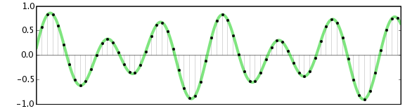
– presentation of a continuous analog signal by means of a sequence of its values (samples). These samples are taken at times separated from each other by an interval called the sampling interval. The reciprocal of the interval between samples is called the sample rate. In Fig. 1 shows the original analog signal and its sampled version. The images below the timing diagrams are obtained assuming that the signals are one line television video signals, the same for the entire television screen.
Analog to digital conversion. Sampling
It is clear that the shorter the sampling interval, and therefore the higher the sampling frequency, the smaller the difference between the original signal and its sampled copy. The stepped structure of the sampled signal can be smoothed with a low-pass filter. This is how the analog signal is restored from the sampled one. But the reconstruction will be accurate only if the sampling frequency is at least 2 times the bandwidth of the original analog signal (this condition is determined by the well-known Kotelnikov theorem). If this condition is not met, the sampling is accompanied by irreversible distortions. The fact is that, as a result of sampling, additional components appear in the frequency spectrum of the signal, which lie around the harmonics of the sampling frequency in the range, equal to twice the bandwidth of the original analog signal. . If the maximum frequency in the frequency spectrum of the analog signal exceeds half the sampling frequency, then the additional components fall within the frequency band of the original analog signal. In this case, it is no longer possible to restore the original signal without distortion. The theory of sampling is covered in many books.
Analog to digital conversion. Distortion sampling
An example of sampling distortions is shown in Fig. 2. An analog signal (again, suppose it is a TV line video signal) contains a wave, the frequency of which first increases from 0.5 MHz to 2.5 MHz and then decreases to 0.5 MHz. This signal is sampled at 3 MHz. In Fig. 2 the images are shown sequentially: the original analog signal, the sampled signal, the restored analog signal after sampling. The low-pass reconstruction filter has a 1.2 MHz bandwidth. As you can see, the low-frequency components (less than 1 MHz) are restored without distortion. The 1.5 MHz wave disappears and becomes a relatively flat field. The 2.5 MHz wave after recovery became a 0.5 MHz wave (this is the difference between the 3 MHz sampling frequency and the original 2.5 MHz frequency). These image diagrams illustrate the distortion associated with an insufficiently high spatial sample rate of the image. If the subject of the television recording is an object that is moving very fast or, for example, a rotating object, then sampling distortions in the time domain may occur. An example of distortion associated with an insufficiently high sample rate (and this is the frame rate of television decay) is an image of a fast moving car on stationary wheels or, for example, slowly turning in one direction or other, the spokes of the wheel (stroboscopic effect). There is no sampling distortion when the bandwidth of the original signal is limited from above and does not exceed half the sampling frequency. associated with insufficiently high spatial sampling rate of the image. If the subject of the television recording is an object that is moving very fast or, for example, a rotating object, then sampling distortions in the time domain may occur. An example of distortion associated with an insufficiently high sample rate (and this is the frame rate of television decay) is an image of a fast moving car on stationary wheels or, for example, slowly turning in one direction or other, the spokes of the wheel (stroboscopic effect). There is no sampling distortion when the bandwidth of the original signal is limited from above and does not exceed half the sampling frequency.
When we talk about the Internet and the current technological “machines” (mobile phone, camera, tablet, computer) we always speak of “digital” and, sometimes, we contrast this term with “analog”. But what exactly these words mean and what they refer to, many times we ignore, perhaps also because it is not relevant for us and is based on being able to use “digital” for what we need without investigating it so much.
“Analog” and “digital” are terms that are constantly encountered when talking about technologies (old and new). In common sense, “analog” is associated with a meaning of “old” or “past” or “low quality”; “Digital”, on the other hand, is synonymous with “new” or “innovative” or “quality”. This common sense distinction is not true.
One thing to keep in mind when addressing these issues is that the definitions of the two terms are one thing (what do they mean, where do they come from, …) and the operational implications they have (because we use one and not the other, as the consequences, implications, results …). As if to say, one thing is the universal law of gravity (with which the sun also has to do) and another is to stay in the sun to warm up and tan.
Another thing to keep in mind is that everything that is under the Digital / Analog issue is not something of our days, its essence was not born with the advent of “new” technologies; here it is one of the oldest problems in human thought and refers to philosophical disquisitions and to the issue of “continuous” and “discrete” variables. But we won’t dwell on these.
As for the definitions. ..
First of all, we must bear in mind that when we talk about Analogue and Digital we refer to ways of representing the measure of a quantity (they are “attributes of a quantity”), to ways in which the quantities we are considering vary (such as a audio signal, a video signal, color,….).
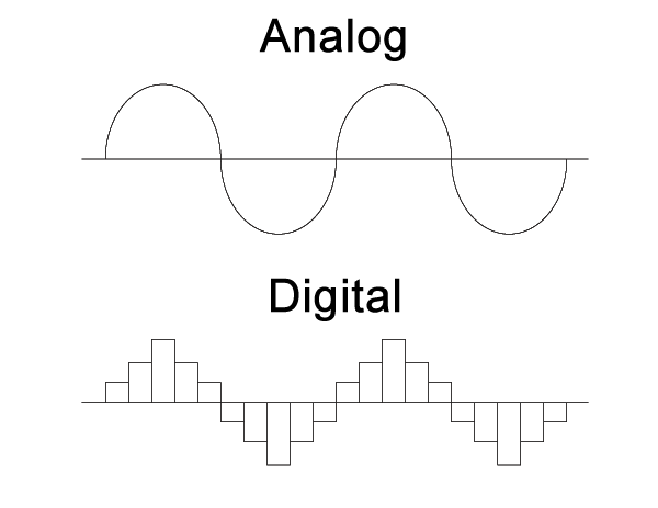
Analogous thing is a continuously varying quantity: an analog variable can take an infinite number of values (for example, the distance between two points in space can take an infinite number of values).
Digital is a quantity that varies “step by step”: a digital variable can take only a finite number of values (the duration of a day; for example, it can take only one of the 85,000 values if we use the “second” unit, a of the 850 thousand values if we use tenths of a second or one of the 8 million and 500 thousand if we use hundredths of a second; many possibilities but still finite, determined).
We can deduce that the concept of analog can be associated with a condition of continuity, that is, in a probable path something moves by changing its location through infinite positions and defining them as infinite we exclude the possibility of being able to number them.
With digital instead, the same path would be divided into stages (steps) and even if it is very small and numerous, it would always be possible to determine the amount.
Practice
Let us now turn to the practical implications of these two ways of representing physical quantities.
Until recently, all the data with which they organized audio or video recordings, static images, data transmissions such as radio, television, telephone were organized in the form of analog signals because the instruments that detected them “. The surfaces” on which they were recorded and the channels through which they were transported were mechanical and made specifically for that type of signal, in fact, they were the same as that signal.
Let’s think about color: the colors we see in a landscape are nothing more than a well-organized set of blue, red and green lights in their infinite shades; its representation through a photograph is based on the combination of blue, red and green pigments (therefore physical objects). We can say that the representation of a landscape through a photographic print is an analog representation of reality.
With the arrival of electronics (which has to do with physical quantities transformed and processed into electrical signals), physical quantities begin to be represented through electrical signals. Initially, these electrical signals were of the analog type (electronics that use continuous signals, signals that can assume an infinite range of possible values, that is, analog signals); later and a special type of signal has been used that can assume only some values among the infinitely possible, in fact it can only assume two values: the presence or absence of the signal. If we look at the basic level of any computer application we will realize that we have a very long series of numbers “one” and “zero” where “one” is the presence of the signal and “zero” its absence.
This is “digital” electronics; digital because it uses signals that are not continuous but “in jumps”.
With the advance of science and technology, both the transmission and recording of analog sounds and images have undergone major changes in recent years. The introduction of digital techniques allows you to do many more things, with greater advantages and more versatility than with analog technology.
Many of the devices that we know today as digital, first receive or capture the signals in analogue form and then convert them into digital signals. This is the case, for example, of CD and DVD players, the modem used by computers for the reception / transmission of data, digital cameras and video cameras, mobile or cell phones, etc.
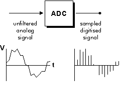
To perform the conversion, these devices use, as an intermediate element, a device called analog-digital converter or ADC (Analogic to Digital Converter), which first receives the electrical signals in the form of an analog sine wave (such as the one provided by the microphone) and It then converts them into digital signals, encoded in binary numerical values, that is, in “zeros” and “ones” (0 – 1).
1. Sound or acoustic wave (voice, music, effects, etc.). 2. Microphone 3. Analog sine wave that is <obtained after the microphone converts the sounds into audio-frequency electrical signals. 4. ADC (Analogic to Digital Converter – Digital Analog Converter). 5. Digital signal formed by zeros and <ones (0 – 1), obtained after the analog signal is processed by the ADC. 6. Output of the <digitized audio signal, ready to be recorded.
In digital cameras and video cameras, as well as in scanners, there is a sensor called CCD (Charge Coupled Device) or, failing that, a CMOS sensor (Complementary Metal Oxide Semiconductor – Semiconductor complementary metal oxide ), which are responsible for converting the images they receive into analog electrical signals.
In that case, as with the microphone, an ADC is responsible for converting those analog signals into digital image signals, so that they can be stored as such in a videotape, on the device’s memory card, or in any other Digital storage device, for later viewing.
The reverse conversion, from digital to analog, is strictly necessary, because the analog sound is the only audible, that is, the only one that recognizes our sense of hearing. Similarly, the analog electrical impulses are the only ones capable of moving the cone of a loudspeaker or loudspeaker to reproduce the original sounds again, which cannot be done by the electrical impulses of “1” and “0” of the binary or digital code. Therefore, to make the coding of the digital sounds audible by the loudspeaker (s), it is necessary to convert them back into analog electrical signals, with their corresponding variations in voltages or voltages.