Tag: is analog or digital signal better

Free Download Mp4Gain

Analog to digital signal conversion Part 3

Keywords can be streamed in parallel or serial.

For parallel transmission, n communication lines must be used (n = 4). The codeword symbols are transmitted simultaneously over the lines within the sampling interval. For serial transmission, the sampling interval must be divided into n subintervals: cycles. In this case, the characters of the word are transmitted sequentially along a line and a clock cycle is assigned for the transmission of one character of the word. Each character of the word is transmitted by one or more discrete signals: pulses. Therefore, converting an analog signal into a sequence of code words is often called pulse code modulation. The way words are represented by certain signals is determined by the format of the code. You can, for example, set the signal level high within the clock cycle if a binary character 1 is transmitted in this clock cycle, and low – if a binary character 0 is transmitted (this representation method, shown in the Fig. 6, it is called BVN format – No return to zero).

In the example of Fig. 6 it uses 4-bit binary words (this allows 16 levels of quantization). In a parallel digital stream, 1 bit of a 4-bit word is transmitted on each line within the sampling interval. In a serial stream, the sampling interval is divided into 4 clocks, in which the bits of a 4-bit word are transmitted (starting with the most significant). 6 uses 4-bit binary words (this allows 16 levels of quantization). In a parallel digital stream, 1 bit of a 4-bit word is transmitted on each line within the sampling interval. In a serial stream, the sampling interval is divided into 4 clocks, in which the bits of a 4-bit word are transmitted (starting with the most significant). 6 uses 4-bit binary words (this allows 16 levels of quantization). In a parallel digital stream, 1 bit of a 4-bit word is transmitted on each line within the sampling interval. In a serial stream, the sampling interval is divided into 4 clocks, in which the bits of a 4-bit word are transmitted (starting with the most significant).

Operations related to converting an analog signal to digital form (sampling, quantizing, and encoding) are performed by one device: an analog-to-digital converter (ADC). Today, an ADC can simply be an integrated circuit. Reverse procedure, ie restoring an analog signal from a sequence of code words is performed in a digital-to-analog converter (DAC). Now there are technical possibilities for implementing all image and sound signal processing, including recording and transmission, in digital form. However, analog devices are still used as signal sensors (for example, a microphone, a TV transmission tube, or a charge-coupled device) and sound and image reproduction devices (for example, a speaker, a kinescope ).

Digital signals can be described using typical parameters of analog technology, such as bandwidth. But its applicability in digital technology is limited. An important indicator characterizing digital flow is the data transfer rate. If the length of the word is n and the sampling rate is FD, then the data rate, expressed in the number of binary symbols per unit time (bit / s), is calculated as the product of the length of the word by the sampling frequency: C = nFD.

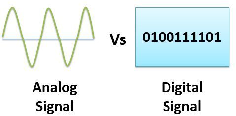
Free Download Mp4Gain


Mp4Gain Main Window


Mp4Gain Features


Free Download Mp4Gain

Analog to digital signal conversion Part 2

If you need no distortion of the TV signal during the sampling process with a cutoff frequency, for example 6 MHz, then the sampling frequency must be at least 12 MHz.

However, the closer the sample rate is to twice the cutoff frequency of the signal, the more difficult it is to create a low-pass filter, which is used in the reconstruction and also in the pre-filtering of the original analog signal. This is due to the fact that as the sampling frequency approaches the doubling cutoff frequency of the sampled signal, increasingly stringent requirements are imposed on the shape of the frequency characteristics of the reconstruction filters: it must correspond more and more precisely to a rectangle. characteristic. It should be noted that a rectangular filter cannot be physically implemented. Such a filter, as theory shows, must introduce an infinitely large delay into the transmitted signal. Therefore, in practice, there is always a certain interval between the doubled cutoff frequency of the original signal and the sampling frequency.

Quantification
– represents the replacement of the count value of the signal with the closest value of a set of fixed values ​​- quantization levels. In other words, quantization is the rounding of the count value. Quantization levels divide the entire range of possible changes in signal values ​​into a finite number of intervals: quantization steps. The location of the quantization levels is determined by the quantization scale. Uniform and non-uniform scales are used. In Fig. 3 shows the original analog signal and its quantized version obtained by means of a uniform quantization scale, as well as the corresponding image signals.

Signal distortions that occur during the quantization process are called quantization noise. In instrumental noise estimation, the difference between the original signal and its quantized copy is calculated and, for example, the root mean square value of this difference is taken as objective noise indicators. The timing diagram and the image of the quantization noise are also shown in Fig. 3 (the image of the quantization noise is shown on a gray background). Unlike jitter noise, quantization noise is correlated with the signal, so quantization noise cannot be removed by post-filtering. The quantization noise decreases as the number of quantization levels increases.

With a relatively large number of levels, the quantization noise is similar to the usual jitter noise. The noise oscillation was reduced, so it was necessary to increase this oscillation 128 times when obtaining an image of quantization noise to make the noise noticeable. A few years ago, it seemed sufficient to use 256 levels to quantify a television video signal. It is now considered the norm to quantify a video signal at 1024 levels. The number of quantization levels in the formation of a digital audio signal is much greater – from tens of thousands to millions.

Digital encoding
A quantized signal, unlike the original analog signal, can only take on a finite number of values. This allows a number equal to the ordinal number of the quantization level to be represented within each sampling interval. In turn, this number can be expressed by a combination of some signs or symbols. The set of characters (symbols) and the system of rules by which data is represented as a set of characters is called a code. The final sequence of code symbols is called a code word. The quantized signal can be converted into a sequence of code words. This operation is called encoding. Each codeword is transmitted within a sampling interval. Binary code is widely used to encode audio and video signals. If the quantized signal can take N values, then the number of binary symbols in each codeword is n> = log2N. A bit, or character in a word represented in binary code, is called a bit. Generally, the number of quantization levels is equal to an integer power of 2, that is, N = 2n.

Analog to digital signal conversion

To convert any analog signal (sound, image) into digital format, three basic operations must be performed: sampling, quantization and encoding.

Sampling
– presentation of a continuous analog signal by means of a sequence of its values ​​(samples). These samples are taken at times separated from each other by an interval called the sampling interval. The reciprocal of the interval between samples is called the sample rate. In Fig. 1 shows the original analog signal and its sampled version. The images below the timing diagrams are obtained assuming that the signals are one line television video signals, the same for the entire television screen.

Analog to digital conversion. Sampling

It is clear that the shorter the sampling interval, and therefore the higher the sampling frequency, the smaller the difference between the original signal and its sampled copy. The stepped structure of the sampled signal can be smoothed with a low-pass filter. This is how the analog signal is restored from the sampled one. But the reconstruction will be accurate only if the sampling frequency is at least 2 times the bandwidth of the original analog signal (this condition is determined by the well-known Kotelnikov theorem). If this condition is not met, the sampling is accompanied by irreversible distortions. The fact is that, as a result of sampling, additional components appear in the frequency spectrum of the signal, which lie around the harmonics of the sampling frequency in the range, equal to twice the bandwidth of the original analog signal. . If the maximum frequency in the frequency spectrum of the analog signal exceeds half the sampling frequency, then the additional components fall within the frequency band of the original analog signal. In this case, it is no longer possible to restore the original signal without distortion. The theory of sampling is covered in many books.

Analog to digital conversion. Distortion sampling

An example of sampling distortions is shown in Fig. 2. An analog signal (again, suppose it is a TV line video signal) contains a wave, the frequency of which first increases from 0.5 MHz to 2.5 MHz and then decreases to 0.5 MHz. This signal is sampled at 3 MHz. In Fig. 2 the images are shown sequentially: the original analog signal, the sampled signal, the restored analog signal after sampling. The low-pass reconstruction filter has a 1.2 MHz bandwidth. As you can see, the low-frequency components (less than 1 MHz) are restored without distortion. The 1.5 MHz wave disappears and becomes a relatively flat field. The 2.5 MHz wave after recovery became a 0.5 MHz wave (this is the difference between the 3 MHz sampling frequency and the original 2.5 MHz frequency). These image diagrams illustrate the distortion associated with an insufficiently high spatial sample rate of the image. If the subject of the television recording is an object that is moving very fast or, for example, a rotating object, then sampling distortions in the time domain may occur. An example of distortion associated with an insufficiently high sample rate (and this is the frame rate of television decay) is an image of a fast moving car on stationary wheels or, for example, slowly turning in one direction or other, the spokes of the wheel (stroboscopic effect). There is no sampling distortion when the bandwidth of the original signal is limited from above and does not exceed half the sampling frequency. associated with insufficiently high spatial sampling rate of the image. If the subject of the television recording is an object that is moving very fast or, for example, a rotating object, then sampling distortions in the time domain may occur. An example of distortion associated with an insufficiently high sample rate (and this is the frame rate of television decay) is an image of a fast moving car on stationary wheels or, for example, slowly turning in one direction or other, the spokes of the wheel (stroboscopic effect). There is no sampling distortion when the bandwidth of the original signal is limited from above and does not exceed half the sampling frequency.