Psychoacoustic Models in MP3 and AAC Encoding


Free Download Mp4Gain
picture

Psychoacoustic Models in MP3 and AAC Encoding

Psychoacoustic Models in MP3 and AAC Encoding

Let’s talk about Psychoacoustic Models in MP3 and AAC Encoding

When it comes to digital audio compression, especially in MP3 and AAC formats, psychoacoustic models are the secret sauce that makes it all work. These models allow us to shrink large audio files into much smaller sizes without a noticeable loss in sound quality. In my years of working with audio encoding, I’ve seen how these models have revolutionized the way we perceive sound after compression. The core idea is simple: we don’t hear all sounds equally. Some frequencies and nuances are more noticeable than others, and psychoacoustic models exploit this fact to make compression more efficient.

Think of it like this: imagine you’re at a concert, and a loud bass guitar is playing alongside a softer violin. Your attention is drawn to the bass because it’s much louder, and the violin’s subtle details get masked. This is exactly what psychoacoustic models do—they remove or reduce sounds that are unlikely to be heard due to masking effects. In this article, I’ll walk you through how psychoacoustic models in MP3 and AAC encoding work and why they matter for audio quality and file size.

Understanding the Basics of Psychoacoustic Models

Psychoacoustic models are based on the science of how our ears and brain perceive sound. They take into account how different sounds mask each other, which frequencies we are most sensitive to, and how we interpret sound in different contexts. MP3 and AAC encoding use these models to compress audio by identifying and removing information that won’t be noticeable to the listener.

A simple analogy would be taking a photograph with a high-resolution camera and then reducing its size by removing some pixels. You won’t notice much difference in the quality of the image because you can’t see all the pixels. Similarly, these audio encoders remove frequencies or audio details that the human ear won’t detect, making the audio file smaller without compromising its perceived quality.

Frequency Masking

  • Frequency masking happens when a louder sound in one frequency range makes a softer sound in a nearby frequency range inaudible.
  • Psychoacoustic models use this to discard or reduce the quieter, masked sounds, optimizing compression.
  • For example, if a heavy guitar is playing at a loud volume, the model might remove the higher-pitched background notes that are masked by the louder guitar.

Temporal Masking

  • Temporal masking occurs when one sound, like a sharp drum hit, can mask a quieter sound that occurs immediately after it.
  • This type of masking is crucial for determining which transient sounds can be removed in compression.
  • For instance, a loud snare hit can mask a subtle violin note that comes milliseconds after, making it unnecessary to keep all the data for that note.

The Role of Psychoacoustic Models in MP3 Encoding

In MP3 encoding, psychoacoustic models play a critical role in reducing the file size while maintaining an acceptable level of sound quality. The MP3 codec was one of the first to use psychoacoustic models to exploit human hearing limitations, and it was revolutionary when it was introduced in the 1990s. The encoder divides audio into different frequency bands and applies masking principles to decide which data can be discarded.

What’s fascinating is that MP3 uses a hybrid of time-domain and frequency-domain processing. It first splits the audio into small segments and then performs a frequency analysis. Using this information, the encoder decides which frequencies can be reduced or eliminated entirely. By doing this, the model allows the MP3 format to achieve relatively small file sizes while preserving the overall listening experience.

MP3 and the Trade-off Between Compression and Quality

  • MP3 encoding sacrifices some of the finer audio details to reduce file size.
  • The trade-off is more noticeable at lower bitrates, where artifacts like compression noise or a “tinny” sound may become audible.
  • Higher bitrates, like 192 kbps or 256 kbps, provide better sound quality, though the file size increases.

AAC: The Next Generation of Psychoacoustic Modeling

While MP3 revolutionized audio compression, AAC (Advanced Audio Codec) takes things a step further. As a more advanced codec, AAC uses a refined psychoacoustic model that performs better at lower bitrates, providing higher-quality audio with less data. This is especially important for modern audio streaming services, which need to balance high-quality sound with efficient bandwidth usage.

The AAC psychoacoustic model is more sophisticated, taking into account additional factors like stereo imaging and spatial effects. It’s also more adept at handling complex audio, such as orchestral music or tracks with a wide range of dynamics. From my experience, AAC does a better job than MP3 in preserving the subtleties of sound, especially at lower bitrates, which is why I recommend it over MP3 when available.

Why AAC Outperforms MP3

  • AAC uses more advanced psychoacoustic techniques, making it more efficient at lower bitrates.
  • It better preserves transient sounds and complex audio elements, like the reverberations of a piano or the nuances of a singer’s voice.
  • With AAC, you can get excellent sound quality at 128 kbps, whereas MP3 may require 192 kbps or higher for a similar result.

How Psychoacoustic Models Help with Audio Quality at Low Bitrates

One of the most remarkable aspects of psychoacoustic models is how they enable high-quality audio at low bitrates. At lower bitrates, many codecs, including MP3 and AAC, might introduce artifacts such as distortion or loss of clarity. However, psychoacoustic models allow the encoder to focus on the most important elements of the sound—those that we are most likely to notice—while discarding the less important parts.

This is especially noticeable in AAC, where the advanced psychoacoustic model ensures that even at low bitrates, the encoding still captures essential auditory information, such as pitch, rhythm, and timbre. I’ve personally found that with AAC, even at 128 kbps, I can enjoy clear vocals and instruments without the harsh artifacts that often accompany MP3 at the same bitrate.

Latest Words on Psychoacoustic Models in MP3 and AAC Encoding

Psychoacoustic models are an integral part of both MP3 and AAC encoding, helping us achieve smaller file sizes while preserving audio quality. These models allow the encoder to reduce the file size by removing sounds that are less perceptible to the human ear, making the audio more efficient without sacrificing what matters most to the listener. While MP3 was groundbreaking in its time, AAC offers superior compression and better handling of complex audio, making it the better choice for modern audio applications.

As I’ve discussed throughout this article, these psychoacoustic models are crucial in ensuring that we can enjoy high-quality audio, even with file sizes that fit comfortably on our devices and bandwidth constraints. Whether you’re listening to your favorite album or streaming a podcast, psychoacoustic models are working behind the scenes to make your audio experience better. As the technology continues to improve, we can only expect even better performance in the future.

Frequently Asked Questions

What are psychoacoustic models in MP3 and AAC encoding?

Psychoacoustic models in MP3 and AAC encoding are based on the way humans perceive sound. These models analyze how different frequencies mask each other, allowing the codecs to remove or reduce the data for sounds that are less noticeable to the human ear. This process helps reduce file size without sacrificing audio quality. Essentially, psychoacoustic models optimize compression by focusing on the most important sounds in an audio file.

How do psychoacoustic models improve audio compression?

Psychoacoustic models improve audio compression by eliminating or reducing sounds that the human ear is less sensitive to. For example, louder sounds can mask softer ones, so the encoder can discard those quieter sounds, saving space without impacting the perceived quality of the audio. This makes it possible to compress audio files into smaller sizes while still delivering high-quality sound, especially in formats like MP3 and AAC.

What is the difference between MP3 and AAC in terms of psychoacoustic models?

The main difference between MP3 and AAC lies in the sophistication of their psychoacoustic models. AAC has a more advanced model that better handles complex audio, such as classical music or tracks with subtle dynamic changes. It also performs better at lower bitrates compared to MP3, providing higher sound quality at the same compression level. In short, AAC offers superior compression efficiency, especially when dealing with modern audio formats and streaming.

Why does AAC sound better than MP3 at lower bitrates?

AAC sounds better than MP3 at lower bitrates because it uses a more efficient psychoacoustic model. The AAC codec is designed to optimize the way it removes or reduces sounds, prioritizing the frequencies that are most important for human perception. This allows it to achieve a better balance between file size and audio quality, especially at bitrates like 128 kbps, where MP3 might begin to show noticeable artifacts.

How does temporal masking affect audio compression?

Temporal masking occurs when a loud sound at one moment in time masks a softer sound that follows it almost immediately. This effect is important for audio compression because it allows the encoder to discard these masked sounds without the listener noticing. This type of masking helps improve compression efficiency, especially in formats like MP3 and AAC, where transient sounds, like a snare hit or cymbal crash, may cover quieter background elements.

Can psychoacoustic models cause distortion in compressed audio?

While psychoacoustic models aim to reduce file size without degrading sound quality, they can sometimes introduce distortion, particularly at lower bitrates. This happens when the codec removes too much data, resulting in noticeable artifacts such as a “tinny” or metallic sound. However, with modern codecs like AAC, these artifacts are much less common, even at lower bitrates, thanks to more advanced psychoacoustic modeling.

Comments:

Wow, I had no idea how much science goes into these audio codecs. Your explanation about frequency and temporal masking really helped me understand why AAC sounds better at lower bitrates. Great article! – AudioFan77

I’ve always been a fan of MP3, but now I’m definitely considering switching to AAC for my music collection. The way you described the differences in psychoacoustic models makes it so much clearer! Thanks! – MusicJunkie88

This article is awesome! The real-life examples helped me visualize how psychoacoustic models work. I never understood how my music could sound so good at a low bitrate, but now I get it. Thanks for the great info! – SoundLover42

Can you talk more about how AAC handles high-frequency sounds compared to MP3? I’d love to know more about that! Great article though, very informative. – HighFreqFan

I didn’t realize how important these psychoacoustic models were in compressing audio. I always wondered how audio streaming services maintain such high-quality sound at lower bitrates. Now I know! – DeeJayDave

This is one of the most detailed articles on this topic I’ve found! I’ve been using AAC for a while now, but this article really made me appreciate how much better it is than MP3, especially for complex audio. – SoundEngineerX

Excellent breakdown of the differences between MP3 and AAC. I always assumed MP3 was “good enough” but now I realize AAC is the better choice, especially for lower bitrates. Thanks for clearing that up! – TechieTom

Great read, but I wish you would’ve gone deeper into how these psychoacoustic models impact the experience for listeners with hearing impairments. Any chance you can dive into that next? – ClearSound76

As a musician, I’ve always been picky about sound quality. After reading this, I’m convinced that AAC is worth the switch for my music files. Thanks for sharing your expertise! – MusicMaker24

I had no idea that psychoacoustic models were so important for compression. I always assumed audio codecs just “squished” the data and that was it! – CuriousGeorge

Very well-written article! I didn’t know much about psychoacoustics before, but now I understand why AAC sounds better at lower bitrates. Thanks for breaking it down so clearly! – TuneInExpert


Free Download Mp4Gain
picture


Mp4Gain Main Window
picture


Mp4Gain Features
picture


Free Download Mp4Gain
picture

Joint Stereo Encoding in MP3

Joint Stereo Encoding in MP3

Joint Stereo Encoding in MP3

Let’s talk about Joint Stereo Encoding in MP3

When we talk about MP3 encoding, joint stereo is one of the most fascinating and efficient techniques used to compress audio files. As someone who’s been working with audio compression for years, I can confidently say that joint stereo plays a pivotal role in optimizing sound quality while reducing file size. This is crucial, especially when you’re dealing with a large collection of music or audio files on your device. For example, think about the way your smartphone stores your favorite playlists. Without joint stereo encoding, those files would take up more space without offering any noticeable improvement in quality.

In essence, joint stereo is a method where the stereo channels (left and right) in a song are not treated as entirely separate entities but are combined in such a way that only the differences between the two are stored. This is like packing the same amount of information into a smaller suitcase without losing any of the essential items. Joint stereo encoding does this by reducing redundancy between the left and right channels, resulting in smaller files with nearly identical sound quality.

It’s important to note that joint stereo encoding is not the same as regular stereo. While regular stereo encoding treats each channel independently, joint stereo takes advantage of the similarities between the two channels to save space. The result is a more efficient encoding process that doesn’t compromise the listener’s experience.

The Mechanics of Joint Stereo Encoding

When we dive deeper into how joint stereo encoding works, it helps to visualize how stereo sound is created. Typically, stereo sound involves two channels: one for the left ear and one for the right ear. However, in many audio tracks, the left and right channels are not radically different from each other. They may have similar instruments, vocals, or background sounds.

What joint stereo encoding does is compare these two channels and only store the parts that differ between them. For the common parts, the encoder only needs to store the data once. This is similar to how two almost identical pictures could be compressed by saving just one of them and recording only the differences for the second one. The result? A significant reduction in file size without a noticeable drop in audio quality.

The Process of Joint Stereo Encoding

  • The encoder analyzes both channels to find similarities and differences.
  • Similar parts of the channels are encoded as a single signal.
  • The differences between the channels are encoded separately, reducing the file size.
  • When decoding, the differences are applied to the common signal, restoring the stereo effect.

By compressing the audio this way, joint stereo encoding ensures that the stereo effect is preserved while minimizing the data needed for storage. This is a significant advantage when you’re trying to fit hundreds or even thousands of songs on a portable device with limited storage capacity.

Types of Joint Stereo Encoding: Mid/Side and Intensity Stereo

There are different types of joint stereo encoding methods that are used depending on the audio track and desired compression level. The two primary types you’ll encounter are Mid/Side (M/S) stereo and Intensity stereo. Both methods offer unique advantages, and understanding these differences is key to choosing the right encoding approach.

Mid/Side Stereo

  • In Mid/Side stereo encoding, the audio is split into two components: the “mid” (center) and the “side” (difference between left and right).
  • The “mid” signal contains information that is common between the left and right channels, while the “side” signal holds the differences.
  • This technique is effective for music that has a strong center sound, like vocals or bass, while allowing the side information to be compressed efficiently.

In my experience, Mid/Side stereo is particularly useful for music with a lot of central elements, like pop or rock tracks where vocals are mixed at the center. By compressing the side channels, the file size shrinks while maintaining clarity in the center of the mix.

Intensity Stereo

  • Intensity stereo encoding focuses on adjusting the volume of the stereo channels based on the perceived loudness of sounds.
  • It reduces the stereo effect for quiet sounds and increases it for louder sounds.
  • This method can save space without compromising the quality of louder parts of the track.

For instance, if you have a song where the guitar solo is prominent, intensity stereo encoding may maintain a full stereo effect for the solo, but reduce the stereo spread during quieter passages, like a soft vocal section. This type of encoding is particularly effective for genres like classical or ambient music, where the dynamic range varies widely throughout the track.

The Advantages of Joint Stereo Encoding

When it comes to audio compression, joint stereo encoding provides several key benefits. I’ve seen firsthand how it allows for more efficient storage without sacrificing the quality that listeners expect from high-quality MP3 files.

Efficient Use of Storage

  • Joint stereo encoding reduces file size significantly by exploiting redundancies between the two channels.
  • This is especially beneficial for users with limited storage space, such as on smartphones or portable music players.
  • Even when file size is reduced, the audio quality remains almost identical to that of traditional stereo encoding.

For example, when I compress a collection of high-quality MP3s for a long road trip, I rely heavily on joint stereo encoding to maximize my storage space. With joint stereo, I’m able to fit hundreds of tracks on my device without having to worry about sound quality degradation.

Sound Quality Preservation

  • Joint stereo encoding preserves the overall sound quality by focusing on the differences between the stereo channels.
  • In contrast to mono encoding, joint stereo ensures that listeners still experience a rich, dynamic soundstage.
  • Most importantly, the compression doesn’t affect the stereo effect that’s essential to enjoying a full, immersive listening experience.

As someone who frequently listens to music on headphones, the stereo effect is crucial to me. I find that even with joint stereo encoding, the balance between left and right channels remains intact, providing an enjoyable experience. It’s remarkable how the technology allows for compression without affecting the auditory experience.

Considerations for Using Joint Stereo Encoding

While joint stereo encoding offers clear benefits, it’s not always the best option for every type of audio. In some situations, particularly with high-fidelity audio or tracks that require precise stereo separation, other encoding methods might be preferable.

High-Fidelity Audio

  • For audiophiles or those with high-end audio equipment, joint stereo encoding may not always be sufficient.
  • The reduced separation between left and right channels can result in a less distinct stereo image.
  • In such cases, lossless encoding or regular stereo encoding might be more suitable to maintain optimal sound quality.

For example, when I listen to classical music or jazz with a wide stereo image, I often opt for uncompressed or higher bit-rate stereo encoding to preserve the detailed spatial arrangement of instruments. Joint stereo, while efficient, may compromise some of the subtle nuances in these genres.

Low-Bitrate Audio

  • At lower bitrates, joint stereo encoding can still provide excellent results in terms of file size reduction without a major loss in quality.
  • However, the compression artifacts may become more noticeable at bitrates lower than 128 kbps.
  • In these situations, a higher bitrate or alternative encoding techniques may be needed to preserve audio fidelity.

If you’re encoding audio for streaming or casual listening, lower bitrates with joint stereo encoding might be a good balance. But when I’m encoding for professional use or high-quality playback, I prefer to use higher bitrates to ensure that the audio remains as close to the original as possible.

Latest Words on Joint Stereo Encoding in MP3

Joint stereo encoding has transformed the way we experience and store audio, offering a balance between quality and compression. Whether you’re a casual listener, a music enthusiast, or a professional audio engineer, understanding the benefits and limitations of joint stereo encoding is crucial for making informed decisions about how you encode and manage your audio files.

With its ability to optimize space and preserve sound quality, joint stereo encoding is one of the most valuable tools in audio compression. As I’ve demonstrated in this article, it’s an essential technique for anyone looking to maximize storage and maintain an excellent listening experience, especially for music that doesn’t rely heavily on complex stereo separation.

While it’s not a one-size-fits-all solution, joint stereo encoding offers significant advantages in most scenarios, particularly for everyday music listening. However, for those with more specialized needs, other encoding methods may be worth exploring. In all cases, it’s important to consider your specific requirements and select the encoding technique that best meets them.

When it comes to MP3 encoding, joint stereo is one of the most effective ways to achieve high-quality audio at a smaller file size, and it remains a staple of audio compression today.

Frequently Asked Questions about Joint Stereo Encoding in MP3

What is Joint Stereo Encoding in MP3?

Joint stereo encoding in MP3 is a compression technique that reduces file size while preserving sound quality. It works by encoding the similarities between the left and right audio channels as a single signal, while only storing the differences separately. This method allows for more efficient use of space without sacrificing the stereo effect, making it ideal for music and audio tracks with similar left and right channels.

How does Joint Stereo Encoding work?

Joint stereo encoding works by analyzing both the left and right channels of audio to identify the parts that are similar. The encoder then stores the common information only once, and the differences between the two channels are encoded separately. When decoding, the differences are applied to the common signal, restoring the full stereo effect for the listener.

What are the different types of Joint Stereo Encoding?

There are two main types of joint stereo encoding: Mid/Side stereo and Intensity stereo. In Mid/Side encoding, the audio is split into a central “mid” signal and a “side” signal that carries the differences between the left and right channels. Intensity stereo adjusts the stereo effect based on the perceived loudness of the audio, reducing the stereo separation for quieter sounds and enhancing it for louder ones.

What are the advantages of using Joint Stereo Encoding?

Joint stereo encoding offers several benefits, including reduced file sizes while maintaining high audio quality. It is especially useful for portable devices with limited storage, as it maximizes space without sacrificing the stereo effect. Joint stereo ensures that audio files retain their immersive listening experience, even at lower bitrates.

Can Joint Stereo Encoding affect audio quality?

At most bitrates, joint stereo encoding does not significantly affect audio quality. However, at lower bitrates, compression artifacts may become noticeable, especially in tracks with complex stereo separation. For high-fidelity audio or genres requiring precise stereo positioning, lossless encoding or standard stereo encoding might be a better option.

Is Joint Stereo Encoding suitable for all types of music?

Joint stereo encoding is highly effective for most types of music, especially tracks where the left and right channels share significant similarities, such as pop, rock, and electronic music. However, for genres like classical or ambient music, where a wide stereo image is essential, other encoding methods or higher bitrates might be preferable to preserve the full stereo effect.

What is the best bitrate for Joint Stereo Encoding?

For most listeners, a bitrate of 128 kbps to 192 kbps is sufficient when using joint stereo encoding. At these bitrates, the file sizes are reduced significantly, while the sound quality remains good. For higher-quality audio, especially in genres where detailed stereo separation is important, higher bitrates such as 256 kbps or 320 kbps are recommended.

How does Joint Stereo Encoding compare to Mono or Stereo Encoding?

Mono encoding combines the left and right channels into a single channel, drastically reducing file size but at the cost of losing the stereo effect. Regular stereo encoding treats both channels independently, resulting in larger file sizes compared to joint stereo. Joint stereo encoding strikes a balance, maintaining a full stereo experience while reducing file size by exploiting the similarities between the two channels.

Comments:

This article really opened my eyes to how joint stereo encoding works. I’ve been using MP3s for years, but I never really understood the technical side of it. Thanks for explaining everything so clearly! – Mike R.

I had no idea about Mid/Side stereo until I read this! It sounds like a great way to compress audio without losing quality. I might try it next time I’m encoding music. – Sarah J.

It’s amazing how joint stereo can save so much space without compromising sound quality. I’ve always used stereo encoding, but now I’m going to give joint stereo a try. – Tom H.

I’ve always wondered why MP3 files are smaller but still sound good. This article explained it perfectly. – Dave L.

I’ve used joint stereo for a while now, but I didn’t realize how much it can impact sound quality at lower bitrates. This article definitely helped me understand it better. – Emily G.

I’ve been encoding a lot of audio for a podcast, and the tips on joint stereo were super helpful. I’m going to implement this on my next set of files. – John K.

Interesting read! I didn’t know that joint stereo could be problematic for audiophiles. I’m going to keep that in mind when working with high-quality audio. – Chris M.

This is one of the most detailed explanations of joint stereo I’ve read. Very helpful! – Jenna T.

Thanks for the insights! I’ve always been curious about how compression works, and now I understand joint stereo much better. – Mark F.

I never realized that the differences between the left and right channels could be compressed so efficiently. I’ll have to try joint stereo next time I encode something. – Alex B.

I appreciate the real-life examples you used. They made the technical details so much easier to understand. – Rick D.

I’ve been having issues with audio quality at low bitrates. This article really helped explain why that happens and how joint stereo can help. – Steve A.

I was always confused about the difference between stereo and joint stereo. This article cleared things up! – Olivia P.

Great breakdown of the different joint stereo types! I’m definitely going to experiment with Mid/Side encoding next time. – Greg W.

MP3 Bit Allocation

What Are the Key Principles Behind MP3 Bit Allocation?

MP3 Bit Allocation
MP3 Bit Allocation

Latest Words on MP3 Bit Allocation

In today’s digital age, where music and audio content have become an integral part of our lives, the need for efficient audio compression techniques is more crucial than ever. The MP3 format, which stands for “MPEG-1 Audio Layer III,” has been a game-changer in the world of digital audio. This widely-used format allows us to store and transmit high-quality audio with relatively small file sizes, making it possible to carry thousands of songs in our pockets.

The magic behind the MP3 format lies in its bit allocation principles. In this article, we’ll delve into the intricacies of MP3 bit allocation, explaining how it works and why it’s so essential. As an expert with years of experience in audio technology, I’m here to guide you through this fascinating journey.

Let’s Talk About MP3 Bit Allocation

MP3 Bit Allocation
MP3 Bit Allocation

Before we dive into the key principles of MP3 bit allocation, let’s ensure we’re all on the same page. You might be wondering what “bit allocation” even means. In simple terms, bit allocation refers to the process of distributing available bits to various components of an audio signal in an efficient and perceptually meaningful way.

Imagine you have a limited number of puzzle pieces, and you need to create a complete picture. Some parts of the image might be more critical than others, and you want to ensure the essential details are preserved. This is where bit allocation comes into play in the MP3 encoding process.

Now, let’s get deeper into the principles behind MP3 bit allocation.

The Psychoacoustic Model: A Vital Component

At the core of MP3 bit allocation is the psychoacoustic model. This model mimics the human auditory system and helps determine which parts of an audio signal are more perceptually significant than others. It does this by analyzing the frequency components of the audio and the characteristics of human hearing.

Imagine you’re in a room filled with people talking at various volumes. Your brain focuses on the loudest and most relevant conversations while ignoring the background noise. Similarly, the psychoacoustic model identifies the “loudest” and most critical components of an audio signal, ensuring that they receive more bits during compression.

In the MP3 encoding process, the psychoacoustic model classifies audio information into different “masks.” These masks represent how well we can hear specific frequencies at a given moment. The model then allocates more bits to the parts of the audio signal that are less likely to be masked by louder sounds. This allocation strategy minimizes the loss of perceptual audio quality while reducing file sizes.

Masking Effect: An Everyday Analogy

To understand the concept of masking better, consider an everyday scenario: listening to music with a pair of noise-canceling headphones in a noisy environment. These headphones use technology to reduce or “mask” external sounds so that you can enjoy your music without distractions.

Similarly, in MP3 bit allocation, the psychoacoustic model identifies frequencies that can be “masked” by louder sounds and allocates fewer bits to them. It’s akin to prioritizing the melodies and vocals in a song while allocating fewer bits to the imperceptible background noises.

This approach is what makes MP3 compression so efficient. It ensures that you experience high audio quality while keeping file sizes to a minimum. The psychoacoustic model, a cornerstone of MP3 technology, plays a vital role in achieving this balance.

The Bit Reservoir: Ensuring Smooth Playback

Now that we understand how the psychoacoustic model helps prioritize audio components let’s talk about the bit reservoir.

Comments:

Comment 1.

I really enjoyed this article! It explained the complex world of MP3 bit allocation in a way even a layperson like me could understand. Great job!

Comment 2.

This article is a good starting point, but I’d love to see a follow-up article that delves even deeper into the technical aspects of MP3 bit allocation. Keep up the good work!

Comment 3.

Kudos to the author for making such a technical topic accessible. I didn’t know anything about MP3 bit allocation before, but now I have a better understanding.

Comment 4.

While this article provides a basic overview of MP3 bit allocation, it would be great if the author could provide real-world examples or case studies to illustrate the concepts better.

Comment 5.

Great explanation! It’s nice to read an article written by someone who knows their stuff. Keep writing more on audio technology, please.

Comment 6.

This article covers the fundamentals well. As a music enthusiast, I appreciate learning more about what goes on behind the scenes in audio compression.

Comment 7.

Wow, I had no idea MP3s were so complex. The part about the psychoacoustic model was fascinating. I look forward to reading more from this author.

Comment 8.

This article could benefit from more practical applications. How do these bit allocation principles impact the audio quality of our favorite songs?

Comment 9.

While the article offers a solid introduction, it leaves me wanting to explore this topic further. It’s a compelling read that piques curiosity.

Comment 10.

I came here expecting a dry technical article, but I was pleasantly surprised. The analogy with noise-canceling headphones was spot on.

Comment 11.

I appreciate the clear and concise language in this article. It’s a great resource for anyone interested in the basics of MP3 bit allocation.

Comment 12.

More, please! I can’t get enough of this topic now. Looking forward to part two. Thanks for making this accessible to the average reader.

Critical Bandwidths in MP3

Calculating Critical Bandwidths in MP3 Compression

Critical Bandwidths in MP3

As an expert in the realm of MP3 compression and audio technology, I’m here to unravel the intricate world of critical bandwidths in MP3 compression. Understanding this concept is pivotal in achieving optimal audio quality while minimizing file size. Let’s dive into the details and explore this fascinating topic.

What Are Critical Bandwidths in MP3 Compression?

Critical bandwidths, often referred to as critical bands, are a fundamental concept in the field of psychoacoustics. They relate to the way our ears perceive different frequencies and play a vital role in audio compression, particularly in the MP3 format. To put it simply, critical bandwidths represent the range of frequencies that our ears can distinguish and process.

Real-Life Example: Think of critical bandwidths as a set of buckets, each representing a range of frequencies. Our ears can only fill a limited number of buckets at once, and these buckets are wider for low frequencies and narrower for high frequencies.

MP3 compression exploits the knowledge of critical bandwidths to remove audio information that falls outside the range of human hearing. This selective approach allows for significant data reduction while retaining audio quality. It’s akin to trimming the fat while preserving the meat, resulting in a leaner audio file.

How Are Critical Bandwidths Determined?

Critical bandwidths are not fixed; they vary depending on the specific frequency and the environment in which the sound is heard. Psychoacoustic studies have led to the development of critical bandwidth curves, which provide a graphical representation of how our ears perceive different frequencies.

Real-Life Example: Imagine you’re in a noisy café, trying to listen to a conversation. Your ears focus on the frequency range of the voices while ignoring the surrounding noise. This selective attention is similar to how critical bandwidths work in audio compression.

In the context of MP3 compression, these critical bandwidth curves are used to determine which parts of the audio spectrum can be discarded without a noticeable impact on the listening experience. This fine-tuned approach ensures that the compression process is both efficient and transparent to our ears.

Balancing Compression and Quality

The art of MP3 compression lies in finding the delicate balance between reducing file size and maintaining audio quality. Critical bandwidths are a crucial tool in achieving this equilibrium. By identifying and preserving the most relevant audio information while discarding what falls outside the critical bandwidths, MP3 compression delivers impressive results.

Real-Life Example: Consider the act of watching a high-definition movie on your smartphone while saving data. The device adjusts the video quality based on the screen size and your internet speed, providing a smooth viewing experience without unnecessary data consumption. MP3 compression operates in a similar fashion, optimizing audio for digital consumption.

In essence, critical bandwidths in MP3 compression serve as a guide to ensure that the compression process is as imperceptible as possible to the human ear. By focusing on the audio information that matters most, we can enjoy high-quality audio experiences with smaller file sizes.

Last Words about Critical Bandwidths in MP3 Compression

In my journey through the realm of audio compression, I’ve come to appreciate the profound impact of critical bandwidths. These frequency ranges shape the way we perceive sound and play a pivotal role in the world of MP3 compression. By understanding this concept, we can navigate the intricacies of audio technology, striking a harmonious balance between quality and efficiency.

Digital audio encoding

Digital audio encoding

Digital audio encoding

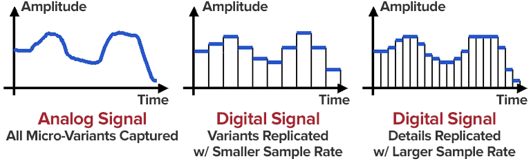
PC-based audio coding is based on the process of converting air vibrations into electrical current fluctuations and the subsequent sampling of an analog electrical signal.

DIGITAL AUDIO ENCODING

The encoding and reproduction of audio information is carried out using special programs. The quality of reproduction of the encoded sound depends on the sampling frequency and its resolution (sound encoding depth – the number of levels).

Digital audio is an analog audio signal represented by discrete numerical values ​​of its amplitude.

Sound digitization is a technology with a divided time step and subsequent recording of the values ​​obtained in numerical form. Another name for digitizing audio is analog to digital audio conversion, which includes the following operations:

Bandwidth limiting is done by using a low pass filter to suppress spectral components that are more than half the sample rate.

Time sampling, that is, replacing a continuous analog signal with a sequence of its values ​​at discrete moments of time: samples.

Level quantization is the replacement of the signal’s reference value with the closest value of a set of fixed values: quantization levels.

Encoding or digitization, as a result of which the value of each quantized sample is represented as a number corresponding to the ordinal number of the quantization level.

This is done as follows: a continuous analog signal is “cut” into sections with a sample rate, a discrete digital signal is obtained, which goes through the quantization process with a certain bit depth, and is then encoded, that is, it is replaced by a sequence of code symbols. To record sound in a 20-20,000 Hz frequency band, a sampling frequency of 44.1 and higher is required (today there are ADCs and DACs with a sampling frequency of 192 and even 384 kHz). To obtain a high-quality recording, 16-bit is sufficient, however, to expand the dynamic range and improve the quality of the sound recording, 24 (less often 32) bits are used.

Sound coding methods (of course an electrical signal coming from a microphone) are based on the fact that, theoretically, any complex sound can be decomposed into a sequence of simpler harmonic signals of different frequencies, each of which it is a sinusoid, called the spectrum of the original signal. The task of encoding sound, like any other analog signal, is to represent it in the form of another analog or digital signal, which is more convenient for its transmission or storage in each specific case. Real sound sources have a limited spectrum width, therefore, for encoding, transformation methods are used that transform the original signal into one, the spectrum of which is more suitable for transmission on the selected channel. Representing an analog signal as another analog signal is commonly referred to as modulation and digitally as encoding. This division is very arbitrary. An analog signal can be represented as a harmonic signal (that is, a sinusoid), the parameters of which change depending on the value of the original signal. In the event that the amplitude of the sinusoid changes with a change in the original signal, it is amplitude modulation (AM). If, depending on the value of the original signal, the frequency or phase of the sinusoid changes, we are dealing with frequency modulation (FM) or phase modulation (PM). Amplitude and frequency modulation, for example, is widely used to transmit sound by radio. These types of modulation, of course, are not the decomposition of the original signal into harmonics. The development of digital technology and the use of computer processing and information storage has led to the widespread use of pulse encoding or modulation methods. Such types of modulation are, for example, pulse code modulation, in which the value of the original signal at regular intervals is represented in code form. The vast majority of “computer sound” is precisely the recording of the binary code of the received signal in short equal time intervals, determined by the sampling frequency. For storage and transmission through communication channels, this signal is usually compressed (reducing the volume by discarding unnecessary or insignificant information). In addition to pulse code modulation, other types of digital modulation (pulse width, pulse frequency, etc.) are also used to encode sound.

Encoding an mp3

Encoding an mp3

encoding mp3

What is masking

mp3 encoding

The lossy MP3 audio compression algorithm uses a limitation of human hearing perception called auditory masking. In 1894, the American physicist Alfred M. Mayer reported that a tone could be made inaudible by another tone of a lower frequency. In 1959, Richard Amer described a complete set of auditory curves related to this phenomenon. Between 1967 and 1974, Eberhard Zwicker worked on tuning and masking critical frequency bands, which in turn built on the fundamental research of Harvey Fletcher and his collaborators at Bell Labs in this area. Perceptual coding was first used to compress speech coding with Linear Prediction Coding (LPC), which has its origins in the works Fuminada Itakura (Nagoya University) and Shuji Saito (from Nippon Telegraph and Telephone) in 1966. In 1978, Bishnu S. Atal and Manfred R. Schroeder of Bell Labs proposed an LPC speech codec called adaptive predictive coding. , which used a psychoacoustic coding algorithm using the masking properties of the human ear. Schroeder and Atal’s further optimization with J.L. Hall was later described in a 1979 article. In the same year M.A. Krasner proposed a psychoacoustic masking codec, which published and produced hardware for speech (not used to compress musical bits), but the publication of its results in a relatively obscure technical report from the Lincoln Laboratory did not immediately influence the mainstream of the development of psychoacoustic codecs. The Discrete Cosine Transform (DCT), a type of transform coding for lossy compression, proposed by Nasir Ahmed in 1972, was developed by Ahmed with T. Natarajan and KR Rao in 1973; published their results in 1974. This led to the development of the Modified Discrete Cosine Transform (MDCT) proposed by JP Princen, AW Johnson, and AB Bradley in 1987 after earlier work by Princen and Bradley in 1986. MDCT later became the main body of the MP3 algorithm. Ernst Terhardt et al. Built an algorithm that describes auditory masking with high precision in 1982. This work adds to many reports by authors dating back to Fletcher, as well as work that originally defined critical ratios and critical bandwidth. In 1985, Atal and Schroeder introduced Code Excited Linear Prediction (CELP), an LPC-based perceptual speech coding auditory masking algorithm that achieved a significant degree of data compression for its time. IEEE peer-reviewed journal “Favorite Communications” reported on a wide variety of audio compression algorithms (mainly perceptual) in 1988. The February 1988 issue of Voice Coding for Communication reported on a wide range of audio compression algorithms bit-based established and operational. technologies, some of which use auditory masking as part of their core design, and some of which show real-time hardware implementations. – https://ru.qaz.wiki/wiki/MP3

ENCODING PRINCIPLES OF THE MP3 FORMAT.

ENCODING PRINCIPLES OF THE MP3 FORMAT.

Mp3 Encoding

Mp3, or fully MPEG-1, 2 and 2.5 Layer 3, is one of the most popular and widespread standards for storing audio data.

MP3 ENCODING

In this article, we will not delve into the history of creation and further development, but will consider the basic principles of the standard and examples of its implementation.

The mp3 standard does not establish a specific compression algorithm to “encode” the source data, but rather describes the essence of the possible methods.

The quality of the result obtained depends on the modification of the algorithm used, embedded in any encoding program of the “codec”, and on the quality of the original audio data.

There are 3 most common modifications of the mp3 format, which differ in the compression ratio parameters of the original audio data.

Name
Modification of the rule
Data rate per second (bit rate) Possible sample rates
MPEG-1 layer 3
32 – 320 kbps 32000 Hz
44100 Hz
48000 Hz
MPEG-2 Layer 3 16 – 160 kbps 16000 Hz
22050 Hz
24000 Hz
MPEG-2.5 Layer 3 8 – up to 160 kbps 8000 Hz
11025 Hz

Processing begins with dividing the original audio signal into equal time intervals: equal frames, for example 0.05 or 0.26 seconds, after which each frame is analyzed and compressed according to general or individual parameters based on the data of the previous and next frames.

Most of the compression algorithms used are based on the perceptual characteristics of the human ear. Let’s consider the main options, which, as a rule, are applied in a complex way.

It is worth starting with the fact that, by ear, the average person is capable of perceiving a frequency range of approximately 10 Hz to 20,000 Hz. With growth, changes occur in the hearing aid and, for most, the sensitivity the higher frequency range decreases, as a result of which, in some mp3 modifications, during compression, all frequencies above 16000 hertz are cut off, which can significantly reduce the amount of information.

Audio recordings can be encoded in stereo (a surround sound effect that uses separate channels for the left and right speakers) or mono (the opposite of stereo). In mp3 format, different tracks are not recorded for each of your speakers, but information about the differences between the left and right channels.

In acoustics, there is a concept like “harmonics”, these are the frequencies of the “sounds” that sound together with the main and most prominent tone. For example, when hitting a drum, the loudest sound will be the tone and the minor, weaker, will be the harmonics.

After such a loud sound, the so-called “period of deafness” occurs, during a period of duration in which a person’s hearing practically does not respond to changes.

If in the intervals of the “deafness period”, remove all frequencies, then the errors of perception, will practically not allow to notice their absence, because of this, during compression, the weakest harmonics are cut off, located close to the most sounds. strong: tones.

A method is used to replace the near peak values ​​of the signal “peaks” (in terms of volume) with an average value.

There is a concept as bit rate: this is a value that characterizes the number of transmitted bits of information “units” during a period of time, usually one second.
The higher the bit rate, the better the audio detail will be, as long as the original, uncompressed audio data is of high quality.

As you can guess, digital formats consist of certain code sequences, in other words of sequences 0 and 1.
To save space, frequent joins within a file are assigned unique identifiers that replace long sequences.

Thanks to such complex influences, it is possible to compress the original audio signal into one of the popular formats with loss of quality – the mp3 format.

Various experiments have been carried out many times in order to reveal how significant the differences are before and after compression in mp3. As tests have shown, differences, some similar moments were not always possible, quickly and to distinguish, even when reproduced on equipment with higher fidelity.

For those who have never had the opportunity to directly compare the original and compressed audio recording, in most cases it will take some time or even find obvious differences.

MP3 ENCODING

MP3 ENCODING

Mp3 encoding

The first step in encoding by the user is to specify a bit rate. This indicates the quality and at the same time the storage requirement of an MP3 file.

MP3 encoding

COMPRESSION RATES

With most recording programs, the quality of an MP3 file can be freely selected before recording begins. According to the Fraunhofer Institute, the CD quality of an MP3 file is a bit rate of 112 to 128 kbit per second, other measurements put CD quality at up to 160 kbit per second. However, the most used and sufficient for most listeners is 128 kbit.

In comparison, a corresponding CD quality for Layer 1 is 384 kbit / s and 256 kbit / s for Layer 2. A wave file works with a 1.4 Mbit / s bit rate and therefore works with roughly the same space requirements. as a CD audio track (CDA).

74 or 80 minutes of music can be put on a CD (depending on the size of the sound carrier), in MP3 format with a bit rate of 128 kbit / s, 11.5 or 12.4 hours would be possible.

PSYCHOACOUSTICS

MP3 audio compression relies on filtering out unnecessary information. Psychoacoustics is a science that deals with the perception of sound by the human ear.

Eg: You are in a disco. Loud music blasts through huge speakers and you try to talk to each other. This is almost impossible unless you yell. In acoustics, this is called masking. To eliminate masking, the sound level of speech should be raised to such an extent that the interfering signal (in this case music) no longer covers it.

Processes like this belong to the fundamental areas of psychoacoustics.

Tones below this threshold are not heard and therefore become noise during MP3 recording (skipped).

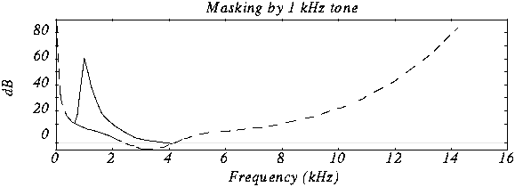
The overlays work as follows: you have, for example (picture 2) a tone with 1 kHz (1) and another tone with 1.1 kHz, which is approximately 18 dB lower (2). The second shade is completely superimposed on the first. This also works for other weaker tones (see Fig. 2). Another tone with a frequency of 2 kHz, which is also 18 dB quieter than the first, would not overlap because it is just outside the threshold of the first tone.

Noise can be another compression option for MP3 recording. The fact that when a sound is digitized it cannot be sampled at an infinite frequency, a noise imperceptible to the human ear (quantization noise) is generated. It is used as a model for the MPEG audio layer and thus increases the noise around a tone. Above all, loud and short tones mask a certain range in the frequency range before and after themselves where the weakest signals would not be audible. With MP3 encoding, the noise level increases in this area, as if digitized at a lower resolution.

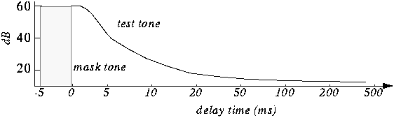
There is also masking in the temporal area: hearing needs a so-called “recovery time” for loud and quiet noises until it is fully functional again. This is especially noticeable with strong, short, and rapidly rising tones. After a delay of about 5 ms, the hearing threshold drops again and after about 200 ms it reaches the normal level, the so-called resting hearing threshold. This effect is called post-masking. The effect of pre-masking is less important, but even more impressive: it is based on the fact that the brain processes loud sounds more quickly than soft ones. To some extent, the strong impulse outweighs the silent one on the way to the brain. This results in a pre-masking time of up to 20 ms.

The above psychoacoustic algorithm is used in the following steps:
– Audio information is divided into subbands
– Subbands are reduced
– 16-bit samples are generated
– Samples are compressed
– Compressed samples are combined into blocks
– Coding according to Huffmann Procedure
: summary in tables

DIVIDED INTO SUBBANDS

Depending on the frequency of the acoustic information, it is divided into 32 subbands. The bands are of different sizes due to adaptation to the human ear according to a psychoacoustic model.

The division is done with the help of a polyphase filter. This means that the samples are decimated and filtered simultaneously.

In layers 1 and 2, the bands were the same size with a bandwidth of 625 Hz each. The reason for this division is to provide the algorithm with a better target.

SUBBAND ​​REDUCTION

The MP3 encoder now examines each of the subbands according to the psychoacoustic model for expendable frequencies. Here, the masking threshold is determined, then the subbands whose level is below this masking function are removed. Another reason for dropping an entire sub-band could be that it is inaudible due to the pitch, similar to a dog’s whistle.

CONVERSION INTO 16-BIT SAMPLES

The frequency bands are sampled and converted to 16-bit samples. Tones are broken down into digital signals and further processed as numerical values. The sample rate determines the length of the sample intervals. However, neither the measurement of the amplitude nor the size of the sampling intervals can be infinitely precise. For this reason, with analog-digital conversion, a value is rounded between two sample points. This results in rounding errors that are noted in what is known as quantization noise. This can be kept inaudible using the highest possible resolution: with 8-bit, a maximum of 256 levels can be displayed, with 12-bit and 4096 and with 16-bit 65536 individual steps, so that noise is not heard.

However, some samples are also digitized with a lower sample rate. In the eighth subband, for example, there is a tone with 1 kHz and 60 dB. The MPEG audio encoder now calculates the masking threshold and recognizes that it is 36dB lower. The acceptable signal-to-noise ratio here is 24 dB, which corresponds to a 4-bit resolution, since the two values ​​are directly related. Leaving one bit out of resolution increases the noise level by 6dB. Since an audio CD is generally digitized with 16 bits, considerable data reduction can be applied here.

SAMPLE COMPRESSION

The next step is to compress the samples further. However, this process no longer has anything to do with the original shades. From here on, compression is only data-driven.

Each sample consists of 16 bits, but not all of them are absolutely necessary to represent a level. For example, leading zeros can be omitted. If, for example, the value 0000011101010101 is obtained for a sample, the algorithm truncates the result to 11101010101. To reconstruct the original 16 bits from this information, the decoder needs two pieces of information: the scale factor and the bit allocation. The scale factor indicates where the remaining bits of the sample were in their original state. The bit mapping contains the information about how many bits are left in the sample, since you can no longer calculate with a fixed 16-bit number. However, if you were to store these values ​​individually for each sample, you wouldn’t gain much,

GROUPING THE SAMPLES

The 16-bit samples that were just created are now combined into blocks. There are two different block lengths for this purpose: the short blocks with twelve samples and the long blocks with 36 samples.

Long blocks are used for low frequencies. However, long blocks would not allow sufficient resolution at higher frequencies; short blocks are used here. In the so-called mixed block mode, long blocks are used for the two frequency bands with the lowest frequencies. For the remaining 30 frequency bands, it is the turn of the short blocks. This mode allows better frequency resolution in the low frequencies without paying tribute to the sampling frequency in the high frequencies.

HUFFMANN CODING

The last step in MP3 compression is Huffmann encoding. This algorithm is also used, for example, in packaging programs such as WinZip. The frequency of certain values ​​is important here. However, the subbands are organized in advance. Subbands with lower frequencies tend to contain significantly more values ​​than those with high frequencies. The subbands are divided into three groups according to their frequency. Each area has its own Huffmann tree (Fig. 3) to achieve the optimal compression factor.

As a first step, the encoder excludes high frequencies; encoding is not necessary here, as its size can be derived from those of the other two regions. The mid-frequency range is treated as is, and the low frequencies are again divided into three regions, each of which is assigned its own Huffmann tree. The appearance of a Huffmann tree is stored in the MP3 file.

The structure of a Huffmann tree works as follows: frequently occurring values ​​are given a short sequence of bits, while rare values ​​are given a long one, so the algorithm first determines the distribution of values ​​within the data to be compressed.

To determine what is known as the Huffman tree, you start with the two rarest values. They are assigned a “0” or a “1”. The two values ​​are summarized, in the order that they are now represented by the sum of their frequency. The same is true for the next two rarer values. This process ends when only one value remains. The result of this procedure is a tree structure. The encoding is based on this structure. Each branch on the left receives a 0, each branch on the right is identified by a “1”. In our little example, the least common would be

Value 4 represented by the sequence of bits 010. The most common value 6, on the other hand, is assigned a simple 1.

FRAMEWORK SUMMARY

The result of the above compression is summarized in so-called frames. Each of these frames contains 1152 samples (32 subbands x 36 samples). A frame consists of a header, a checksum check, the actual audio data, and in certain circumstances a so-called bit repository. Such a deposit arises when the samples within the frame can be compressed in such a way that the full theoretical number of bits in a frame is not required. The encoder can fall back on these buckets if the available bits are insufficient for a subsequent frame. A distinction must be made between two terms: frame size and frame length.

The size of the frame is determined by the number of samples and is constant within a layer. In Layer 1 format, this is always 384 samples per frame, in Layers 2 and 3 1152 per frame. However, the length of the frame may differ at Layer 3 due to the change in bit rate or the pool of unfilled bits. The frame also contains the aforementioned information about the scale factor and bit allocation to be able to reconstruct all the samples again.

A file header, as it is known from other file formats, does not exist in an MP3 file. In the case of an image file, a header would contain information about the entire image (e.g. size, color depth, resolution

MP3 COMPRESSION

MP3 COMPRESSION

To achieve such a dramatic reduction in the number of bits required to transmit an MP audio signal, use different techniques. These techniques include those based on perceptual coding and others such as byte reservation, stereo assembly or Huffman codes. Percentage coding consists of removing all the information that goes into the audio signal that the human ear is not capable of detecting. We will now describe them:

PERCEPTUAL CODING

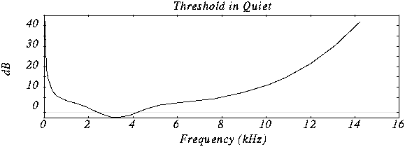
Minimum hearing threshold The ear’s minimum hearing threshold is the power below which a tone at a given frequency is not capable of being detected by the ear. This threshold is non-linear. As we see in the figure, which represents the Fletcher and Mundson law, the frequencies in which we hear best are those between 2 and 5 Khz. Therefore frequencies outside that band are not totally essential since they will hardly be perceived. Therefore it is possible to remove the content of the audio signal outside these frequencies.

As we can see in the drawing, the range in which a lower power is needed for the tone to be heard is between 2 and 4 Khz.

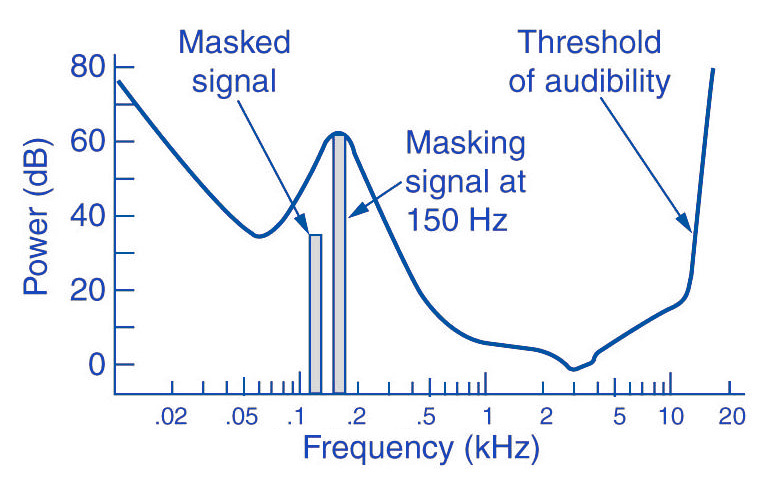
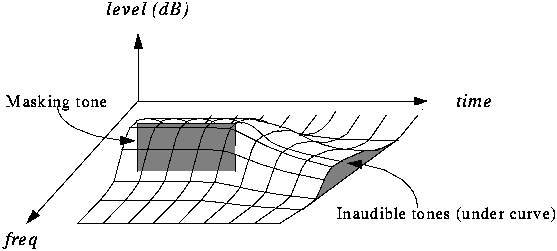
The masking effect This effect consists in that, when an audio signal has a tone at a given frequency, it produces a masking effect at the frequencies close to it, so that if at these nearby frequencies the signal does not exceed a certain power threshold cannot be heard and therefore it is not necessary to encode them. The form that this power threshold will take according to the position of the tone or the masking tones is what is called the psychoacoustic model, which as the name itself indicates is a perception model that tries to emulate the perception of the human ear.

In this graph we can see how if we put a tone at 1 Khz of 60 dB (masking tone) and then we put another tone at, for example 1.1 Khz and we vary the frequency of this, it is not possible to detect the presence of this second tone until its power exceeds the threshold presented in the figure.

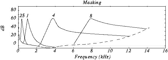
In this case we see various masking tones and the resulting new hearing thresholds. In MP3, what is done is to divide the spectrum to be transmitted (that is, between 2 and 5 Khz) into frequency subbands, so that the power of the subband is evaluated and the masking threshold is created in the nearby subbands. Nearby subbands that exceed that power threshold are coded and those that do not exceed it are not coded.

Furthermore, the masking is not only in appearance but also in time as we can see in the figure.

The byte reserve: Often, some passages of a musical piece cannot be encoded at the same rate without altering the quality of the music. MP · then uses a small byte reservation that acts as a buffer using the capacity of passages that can be encoded at a lower rate in the given stream.
The stereo assembly In the case of a stereo signal, the MP3 format can use a few more tools to further compress the data.
Intensity stereo (IS) The human ear is not able to locate with complete certainty the spatial origin of sounds for very high or very low frequencies. This technique takes advantage of this, recording some frequencies as a monophonic signal, so that a minimum of spatial content is subtracted from the sound.
Mid / Side (M / S) Stereo When the left and right channels are similar then a middle channel (L + R) and a side channel (LR) are created, which are encoded instead of encoding the left channel on one side and the right for another. In this way it is possible to reduce the transmitted data using fewer bits for the lateral channel. Then during playback the MP3 decoder will reconstruct the left and right channels.

Huffman Coding: This coding technique is used at the end of the whole process. It works by creating variable-length codes, so that the symbols that appear in the bitstream most likely have shorter codes. The translation between symbols and codes is done using a table. Each code has a unique prefix so that the codes can be decoded correctly despite their variable length. This type of coding allows on average to reduce by 20% the amount of data to be transmitted. It is an ideal complement to perceptual coding since, during great polyphonies, perceptual coding is very efficient since many sounds are masked, but nevertheless little information is identical and Huffman’s algorithm becomes inefficient. During pure sounds there are few masking effects, but Huffman encoding is very efficient since digitized sound contains many repeating bytes.