MP3 ENCODING
The first step in encoding by the user is to specify a bit rate. This indicates the quality and at the same time the storage requirement of an MP3 file.

COMPRESSION RATES
With most recording programs, the quality of an MP3 file can be freely selected before recording begins. According to the Fraunhofer Institute, the CD quality of an MP3 file is a bit rate of 112 to 128 kbit per second, other measurements put CD quality at up to 160 kbit per second. However, the most used and sufficient for most listeners is 128 kbit.
In comparison, a corresponding CD quality for Layer 1 is 384 kbit / s and 256 kbit / s for Layer 2. A wave file works with a 1.4 Mbit / s bit rate and therefore works with roughly the same space requirements. as a CD audio track (CDA).
74 or 80 minutes of music can be put on a CD (depending on the size of the sound carrier), in MP3 format with a bit rate of 128 kbit / s, 11.5 or 12.4 hours would be possible.
PSYCHOACOUSTICS
MP3 audio compression relies on filtering out unnecessary information. Psychoacoustics is a science that deals with the perception of sound by the human ear.
Eg: You are in a disco. Loud music blasts through huge speakers and you try to talk to each other. This is almost impossible unless you yell. In acoustics, this is called masking. To eliminate masking, the sound level of speech should be raised to such an extent that the interfering signal (in this case music) no longer covers it.
Processes like this belong to the fundamental areas of psychoacoustics.
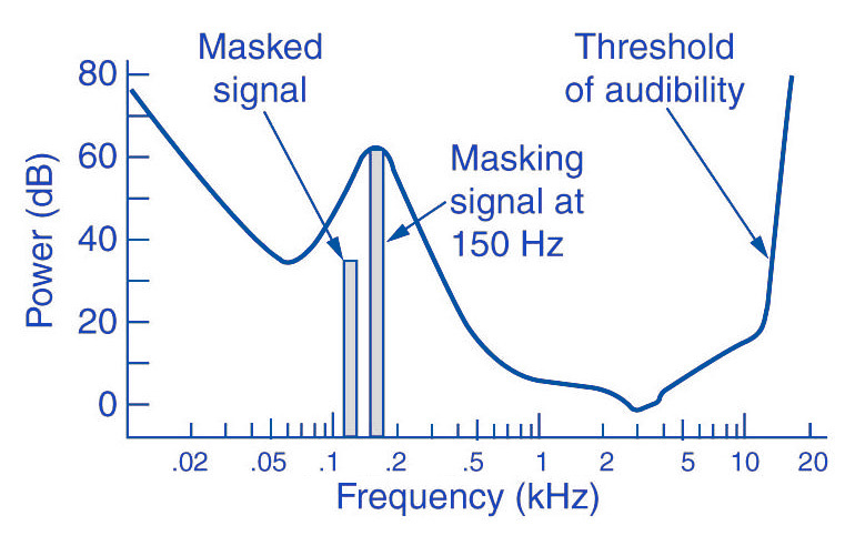
Tones below this threshold are not heard and therefore become noise during MP3 recording (skipped).
The overlays work as follows: you have, for example (picture 2) a tone with 1 kHz (1) and another tone with 1.1 kHz, which is approximately 18 dB lower (2). The second shade is completely superimposed on the first. This also works for other weaker tones (see Fig. 2). Another tone with a frequency of 2 kHz, which is also 18 dB quieter than the first, would not overlap because it is just outside the threshold of the first tone.
Noise can be another compression option for MP3 recording. The fact that when a sound is digitized it cannot be sampled at an infinite frequency, a noise imperceptible to the human ear (quantization noise) is generated. It is used as a model for the MPEG audio layer and thus increases the noise around a tone. Above all, loud and short tones mask a certain range in the frequency range before and after themselves where the weakest signals would not be audible. With MP3 encoding, the noise level increases in this area, as if digitized at a lower resolution.
There is also masking in the temporal area: hearing needs a so-called “recovery time” for loud and quiet noises until it is fully functional again. This is especially noticeable with strong, short, and rapidly rising tones. After a delay of about 5 ms, the hearing threshold drops again and after about 200 ms it reaches the normal level, the so-called resting hearing threshold. This effect is called post-masking. The effect of pre-masking is less important, but even more impressive: it is based on the fact that the brain processes loud sounds more quickly than soft ones. To some extent, the strong impulse outweighs the silent one on the way to the brain. This results in a pre-masking time of up to 20 ms.
The above psychoacoustic algorithm is used in the following steps:
– Audio information is divided into subbands
– Subbands are reduced
– 16-bit samples are generated
– Samples are compressed
– Compressed samples are combined into blocks
– Coding according to Huffmann Procedure
: summary in tables
DIVIDED INTO SUBBANDS
Depending on the frequency of the acoustic information, it is divided into 32 subbands. The bands are of different sizes due to adaptation to the human ear according to a psychoacoustic model.
The division is done with the help of a polyphase filter. This means that the samples are decimated and filtered simultaneously.
In layers 1 and 2, the bands were the same size with a bandwidth of 625 Hz each. The reason for this division is to provide the algorithm with a better target.
SUBBAND REDUCTION
The MP3 encoder now examines each of the subbands according to the psychoacoustic model for expendable frequencies. Here, the masking threshold is determined, then the subbands whose level is below this masking function are removed. Another reason for dropping an entire sub-band could be that it is inaudible due to the pitch, similar to a dog’s whistle.
CONVERSION INTO 16-BIT SAMPLES
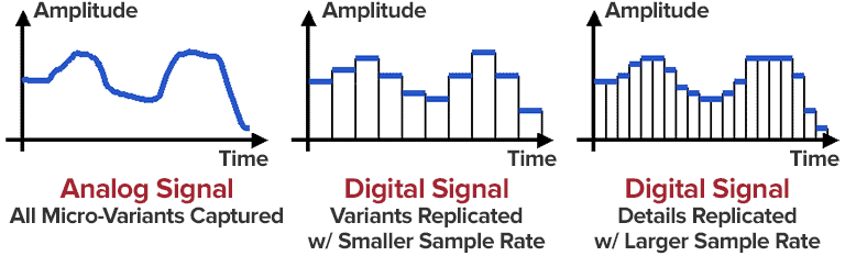
The frequency bands are sampled and converted to 16-bit samples. Tones are broken down into digital signals and further processed as numerical values. The sample rate determines the length of the sample intervals. However, neither the measurement of the amplitude nor the size of the sampling intervals can be infinitely precise. For this reason, with analog-digital conversion, a value is rounded between two sample points. This results in rounding errors that are noted in what is known as quantization noise. This can be kept inaudible using the highest possible resolution: with 8-bit, a maximum of 256 levels can be displayed, with 12-bit and 4096 and with 16-bit 65536 individual steps, so that noise is not heard.
However, some samples are also digitized with a lower sample rate. In the eighth subband, for example, there is a tone with 1 kHz and 60 dB. The MPEG audio encoder now calculates the masking threshold and recognizes that it is 36dB lower. The acceptable signal-to-noise ratio here is 24 dB, which corresponds to a 4-bit resolution, since the two values are directly related. Leaving one bit out of resolution increases the noise level by 6dB. Since an audio CD is generally digitized with 16 bits, considerable data reduction can be applied here.
SAMPLE COMPRESSION
The next step is to compress the samples further. However, this process no longer has anything to do with the original shades. From here on, compression is only data-driven.
Each sample consists of 16 bits, but not all of them are absolutely necessary to represent a level. For example, leading zeros can be omitted. If, for example, the value 0000011101010101 is obtained for a sample, the algorithm truncates the result to 11101010101. To reconstruct the original 16 bits from this information, the decoder needs two pieces of information: the scale factor and the bit allocation. The scale factor indicates where the remaining bits of the sample were in their original state. The bit mapping contains the information about how many bits are left in the sample, since you can no longer calculate with a fixed 16-bit number. However, if you were to store these values individually for each sample, you wouldn’t gain much,
GROUPING THE SAMPLES
The 16-bit samples that were just created are now combined into blocks. There are two different block lengths for this purpose: the short blocks with twelve samples and the long blocks with 36 samples.
Long blocks are used for low frequencies. However, long blocks would not allow sufficient resolution at higher frequencies; short blocks are used here. In the so-called mixed block mode, long blocks are used for the two frequency bands with the lowest frequencies. For the remaining 30 frequency bands, it is the turn of the short blocks. This mode allows better frequency resolution in the low frequencies without paying tribute to the sampling frequency in the high frequencies.
HUFFMANN CODING
The last step in MP3 compression is Huffmann encoding. This algorithm is also used, for example, in packaging programs such as WinZip. The frequency of certain values is important here. However, the subbands are organized in advance. Subbands with lower frequencies tend to contain significantly more values than those with high frequencies. The subbands are divided into three groups according to their frequency. Each area has its own Huffmann tree (Fig. 3) to achieve the optimal compression factor.
As a first step, the encoder excludes high frequencies; encoding is not necessary here, as its size can be derived from those of the other two regions. The mid-frequency range is treated as is, and the low frequencies are again divided into three regions, each of which is assigned its own Huffmann tree. The appearance of a Huffmann tree is stored in the MP3 file.
The structure of a Huffmann tree works as follows: frequently occurring values are given a short sequence of bits, while rare values are given a long one, so the algorithm first determines the distribution of values within the data to be compressed.
To determine what is known as the Huffman tree, you start with the two rarest values. They are assigned a “0” or a “1”. The two values are summarized, in the order that they are now represented by the sum of their frequency. The same is true for the next two rarer values. This process ends when only one value remains. The result of this procedure is a tree structure. The encoding is based on this structure. Each branch on the left receives a 0, each branch on the right is identified by a “1”. In our little example, the least common would be
Value 4 represented by the sequence of bits 010. The most common value 6, on the other hand, is assigned a simple 1.
FRAMEWORK SUMMARY
The result of the above compression is summarized in so-called frames. Each of these frames contains 1152 samples (32 subbands x 36 samples). A frame consists of a header, a checksum check, the actual audio data, and in certain circumstances a so-called bit repository. Such a deposit arises when the samples within the frame can be compressed in such a way that the full theoretical number of bits in a frame is not required. The encoder can fall back on these buckets if the available bits are insufficient for a subsequent frame. A distinction must be made between two terms: frame size and frame length.
The size of the frame is determined by the number of samples and is constant within a layer. In Layer 1 format, this is always 384 samples per frame, in Layers 2 and 3 1152 per frame. However, the length of the frame may differ at Layer 3 due to the change in bit rate or the pool of unfilled bits. The frame also contains the aforementioned information about the scale factor and bit allocation to be able to reconstruct all the samples again.
A file header, as it is known from other file formats, does not exist in an MP3 file. In the case of an image file, a header would contain information about the entire image (e.g. size, color depth, resolution