Audio and video Archives - Page 133 of 196

What interfaces are used for digital audio transmission?

Free Download Mp4Gain

What interfaces are used for digital audio transmission?

Digital Audio Transmission

S / PDIF (Sony / Phillips Digital Interface Format, a Sony and Phillips digital interface format) is a digital interface for consumer radio equipment.

AES / EBU (Audio Engineers Society / European Broadcast Union) is a digital interface for studio radio equipment.

Both interfaces are serial and use the same signal format and coding system, BMC (biphasic mark code) with automatic synchronization and can transmit signals in PCM format of up to 24 bits at sample rates up to 48 kHz.

Each sample of the signal is transmitted as a 32-bit word, in which 20 bits are used to transfer the sample and 12 bits to form the sync preamble, transfer additional information, and the parity bit. The 4 bits of the overload group can be used to expand the sample format to 24 bits.

In addition to the parity bit, the word overhead contains the validity bit, which must be zero for each valid sample. In the case of receiving a word with a single bit of Validity or with a parity violation in the word, the receiver interprets the entire sample as wrong and can choose to replace it with the previous value or interpolate based on several adjacent valid samples. Invalid readings can be transmitted by CD players, DAT recorders and other devices, if during the reading of the carrier information it was not possible to correct the errors that occurred during the reading process.

As a standard, the encoding format is intended for the transmission of a one and two channel signal; however, when the service bits are used to encode a channel number, a multi-channel signal can be transmitted.

On the electrical side, S / PDIF allows connection with a coaxial cable with a characteristic impedance of 75 Ohm and RCA connectors (“tulip”), the amplitude of the signal is 0.5 V. AES / EBU allows connection with a two-wire shielded symmetrical cable with transformer isolation through the RS-422 interface with a signal amplitude 3-10 V, connectors – three-pin XLR Cannon type. There are also options for optical transceivers: TosLink (plastic fiber) and AT&T Link (fiberglass).

Free Download Mp4Gain

Mp4Gain Main Window

Mp4Gain Features

Free Download Mp4Gain

What are the pros and cons of digital audio?

What are the pros and cons of digital audio?

Digital Audio

The digital representation of sound is valuable, first of all, for the possibility of endless storage and reproduction without loss of quality; however, the conversion from analog to digital and vice versa inevitably leads to its partial loss.

digital audio

The most unpleasant distortions introduced in the digitizing stage are the granular noise that occurs when the signal is quantized by level due to rounding of the amplitude to the nearest discrete value. Unlike simple broadband noise introduced by quantization errors, granular noise is the harmonic distortion of the signal, most noticeable in the upper part of the spectrum.

The power of the granular noise is inversely proportional to the number of quantization steps; However, due to the logarithmic characteristic of hearing with linear quantization (constant step value), quiet sounds have fewer quantization steps than loud sounds, and as a result, the main density of non-linear distortions falls in the region of sounds. silent. This leads to a limitation of the dynamic range, which ideally (without taking into account harmonic distortion) would be equal to the signal-to-noise ratio, but the need to limit this distortion reduces the dynamic range for 16-bit encoding to 50-60 dB. The situation could have been saved by logarithmic quantification, but its implementation in real time is very difficult and expensive.

The distortion introduced by granular noise can be reduced by adding normal white noise (random or pseudo-random signal) to the signal, with an amplitude of half the least significant bit; such an operation is called dithering. This leads to a slight increase in the noise level, but weakens the correlation of quantization errors with the components of the high-frequency signal and improves subjective perception. Anti-aliasing is also applied before rounding the samples by decreasing their bit depth. Essentially, dithering and noise shaping are special cases of the same technology, with the difference that, in the first case, white noise with a flat spectrum is used and, in the second, noise with a spectrum with a “shape “special.

When restoring audio from digital to analog, there is the problem of smoothing the stepped waveform and suppressing the harmonics introduced by the sample rate. Due to the imperfection of the frequency response of the filters, insufficient suppression of this interference or excessive attenuation of useful high-frequency components may occur. Poorly suppressed sample rate harmonics distort the shape of the analog signal (especially in the high frequency region), resulting in a “rough” and “dirty” sound.

How do ADCs and DACs work and function?

How do ADCs and DACs work and function?

ADC and DAC

There are mainly three ADC designs:

ADC DAC

Parallel – The input signal is simultaneously compared to the reference levels by a set of comparison circuits (comparators), which form a binary value at the output. In such ADC, the number of comparators is equal to (2 to the power N) – 1, where N is the digit capacity of the digital code (for an eight-bit code – 255), which does not allow to increase the capacity of digits above 10-12.
Successive approximation: The converter using an auxiliary DAC generates a reference signal that is compared to the input signal. The reference signal is changed sequentially according to the principle of mean division (dichotomy), which is used in many convergent search methods in applied mathematics. This makes it possible to complete the conversion in a number of clock cycles equal to the length of the word, regardless of the size of the input signal.
with time interval measurement: a large group of ADCs that use various principles of converting levels into proportional time intervals to measure the input signal, the duration of which is measured by a high frequency clock generator. This is sometimes called ADC counting.
Among ADCs with time interval measurement, the following three types prevail:

Sequential Count or Single Slope – In each conversion cycle, a linearly increasing voltage generator is started, which is compared to the input voltage. Typically this voltage is obtained from an auxiliary DAC, similar to a successive approximation ADC.
Dual Slope: In each conversion cycle, the input signal charges a capacitor, which is then discharged to a reference voltage with the duration of discharge measured.
tracking – A variant of the sequential counting ADC, in which the reference voltage generator does not reset on each cycle, but instead changes it from the previous value to the current one.
The most popular version of the tracking ADC is sigma-delta, which operates at a frequency Fs, which is significantly (64 times or more) higher than the sampling frequency Fd of the digital output signal. The comparator of such an ADC produces values of reduced bit depth (generally a bit – 0/1), the sum of which in the sampling interval Fd is proportional to the value of the sample. A sequence of low bit values is digitally filtered and decimated, resulting in a series of samples with a given bit depth and sample rate Fd.

To improve the signal-to-noise ratio and reduce the effect of quantization errors, which in the case of a one-bit converter turns out to be quite high, a noise shaping method is used through digital filtering and feedback circuits. error. As a result of applying this method, the shape of the noise spectrum changes so that the main noise energy is shifted to the region above the middle of the frequency Fs, a small part remains in the lower half, and almost all the noise it is removed from the original analog signal band.

DACs are based primarily on three principles:

weighting: with the sum of the weighted currents or voltages, when each bit of the input word makes a contribution corresponding to its binary weight to the total value of the received analog signal; These DACs are also called parallel or multibit (multibit).
sigma-delta, with preliminary digital oversampling and delivery of low-bit (usually one-bit) values to the reference charge-shaping circuit, which are added to the output signal with the same high frequency. These DACs are also called bit streams.
Pulse Width Modulation (PWM), when pulses of constant amplitude and variable duration are sent to the analog sample and hold signal, controlling the dosage of the load discharged at the output. Matsushita’s MASH (Multi-stAge Noise Shaping) converters work with this principle. These DACs got their name due to the use of various sequential noise shapers in them.
When using oversampling by a factor of tens (typically – 64x..512x), it is possible to reduce the DAC capacity without noticeable loss of signal quality; DACs with fewer bits also have better linearity. At the limit, the number of downloads can be reduced to one. The output waveform of such DACs is a useful signal surrounded by a significant amount of high frequency noise, which, however, is effectively suppressed by a uniform medium quality analog filter.

DACs are “straightforward” devices where conversion is easier and faster than ADCs, which are mostly slower and serial devices.

What is oversampling?

What is oversampling?

It involves sampling the signal at a rate higher than the base sample rate. Oversampling can be analog, when sampling the original signal at an increased frequency, or digital, when additional samples calculated by interpolation are inserted between existing digital samples. Another way to get intermediate sample values is to insert zeros, after which the entire sequence is digitally filtered. The ADC uses analog oversampling, the DAC uses digital.

Oversampling is used to simplify ADC and DAC designs. According to the problem conditions, an analog filter with a linear AFC in the operating range and steeply falling out of it should be installed at the input of the ADC and the output of the DAC. The implementation of an analog filter of this type is quite complex; at the same time, when the sampling frequency is increased, the reflections of the spectrum introduced by it are compensated proportionally with respect to the main signal and the analog filter can have a much lower cutoff slope.

Another advantage of oversampling is that the amplitude quantization errors (squash noise) distributed over the entire spectrum of the signal being quantized are spread over a wider bandwidth when sampling, so there is less noise present. on the main audio signal. Each frequency doubling reduces the quantization noise level by 3 dB; Since one bit equals 6 dB of noise, each quadruple of the frequency reduces the converter’s capacity by one.

Oversampling, coupled with an increase in the sample bit depth, interpolation of the samples with greater precision, and their output to a DAC of the appropriate bit depth, allows for some improvement in the reconstruction quality of the audio signal. For this reason, even 16-bit systems often use 18- and 20-bit oversampling DACs.

Oversampling ADCs and DACs can do without sample and hold circuitry by significantly reducing conversion time.

What is Analog-to-Digital and Digital-to-Analog Converters (ADC and DAC)?

What is Analog-to-Digital and Digital-to-Analog Converters (ADC and DAC)?

Analog to Digital

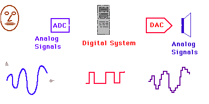
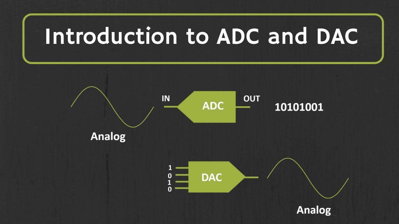
Analog-to-digital and digital-to-analog converters. The first converts the analog signal into a digital value of the amplitude, the second performs the inverse conversion. In the English language literature, the terms ADC and DAC are used, and the combined converter is called a codec (codec).

Digital and Analog

The working principle of the ADC is to measure the level of the input signal and output the result in digital form. As a result of ADC operation, a continuous analog signal is converted to a pulse signal, with a simultaneous measurement of the amplitude of each pulse. The DAC receives a digital value of the amplitude at the input and outputs voltage or current pulses of the required magnitude at the output, which the integrator (analog filter) located behind it converts into a continuous analog signal.

In order for the ADC to function properly, the input signal must not change during the conversion time, so a sample hold circuit is usually placed at its input, which captures the instantaneous signal level and holds it for the entire time. Of conversation. A similar circuit can also be installed at the DAC output, suppressing the effect of transient processes within the DAC on the output signal parameters.

With time sampling, the spectrum of the pulse signal received in its lower part 0..Fa repeats the spectrum of the original signal, and above it contains a series of reflections (aliases, mirror spectra), which are located around the sampling frequency Fd and its harmonics (sidebands). In this case, the first reflection of the spectrum from the frequency Fd in the case of Fd = 2Fa is located directly behind the original signal band, and requires an analog filter (anti-alias filter) with a high cutoff slope to delete it. In the ADC, this filter is installed at the input to eliminate spectral overlap and its interference, and in the DAC, at the output, to suppress the supra-tone noise introduced by time sampling in the output signal.

How is sound represented digitally?

How is sound represented digitally?

Digital Representation of Sound

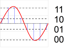
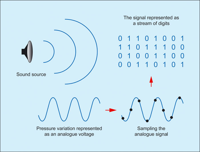
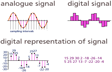
The original shape of an audio signal (a continuous change in amplitude over time) is represented digitally by “cross-sampling”, in time and level.

Representing Sound Digitally

According to Kotelnikov’s theorem, any continuous process with a limited spectrum can be completely described by a discrete sequence of its instantaneous values, following with a frequency at least twice the frequency of the highest harmonic of the process; the sampling frequency Fd of instantaneous values (samples) is called the sampling frequency.

It follows from the theorem that a signal with a frequency Fa can be successfully sampled in time at a frequency 2Fa only if it is a pure sinusoid, because any deviation from the sinusoidal shape leads the spectrum to go beyond the frequency Fa. Therefore, for temporal sampling of an arbitrary audio signal (which normally has, as is known, a spectrum that falls smoothly), it is necessary to select a sampling frequency with a margin or to forcefully limit the spectrum of the input signal below half the sample rate.

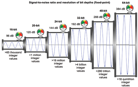
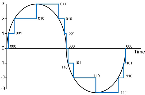
Simultaneously with time sampling, amplitude sampling is performed: measurement of instantaneous amplitude values and their representation in the form of numerical values with some precision. The precision of the measurement (binary width N of the obtained discrete value) determines the signal-to-noise ratio and the dynamic range of the signal (theoretically these are reciprocal values, but any real path also has its own level of noise and interference).

The resulting stream of numbers (a series of binary digits) that describe an audio signal is called Pulse Code Modulation (PCM), since each pulse of a time-sampled signal is represented by its own digital code.

Linear quantization is most often used when the numerical value of the sample is proportional to the amplitude of the signal. Due to the logarithmic nature of hearing, logarithmic quantization, when the numerical value is proportional to the magnitude of the signal in decibels, would be more appropriate, but this is fraught with difficulties of a purely technical nature.

Time sampling and amplitude quantization of the signal inevitably introduce noise distortions in the signal, the level of which is generally estimated using the formula 6N + 10lg (Fdiscr / 2Fmax) + C (dB), where the constant C varies for different types of signals: for a pure sinusoid it is 1.7 dB, for sound signals – from -15 to 2 dB. Thus, it can be seen that a decrease in noise in the operating frequency band 0..Fmax leads not only to an increase in the bit depth of the sample, but also to an increase in the sample rate relative to 2Fmax, as the quantization noise is “smeared” across the band up to the sample rate, and the audio information occupies only the smallest part of this strip.

Most modern digital audio systems use the standard 44.1 and 48 kHz sample rates, but the frequency range of the signal is usually limited to about 20 kHz to keep it clear of the theoretical limit. Also the most common is 16-bit level quantization, which provides a limit signal-to-noise ratio of approximately 98 dB. The studio equipment uses higher resolutions: 18, 20, and 24-bit quantization at 56, 96, and 192 kHz sample rates. This is done to preserve the higher harmonics of the sound signal, which are not directly perceived by the ear, but affect the formation of the overall sound image.

To digitize lower-quality, narrow-band signals, you can lower the sample rate and bit depth; for example, telephone lines use 7 or 8 bit digitization with frequencies 8..12 kHz.

The representation of an analog signal in digital form is also called Pulse Code Modulation (PCM), since the signal is represented as a series of pulses of constant frequency (time sampling), the amplitude of which is transmitted digitally (amplitude sampling ). A PCM stream can be parallel, when all the bits in each sample are transmitted simultaneously over several lines with one sampling frequency, or sequential, when the bits are transmitted one after another at a higher frequency on a line.

Digital sound itself and related elements are often denoted by the general term Digital Audio; The analog and digital portions of a sound system are called the Analog Domain and Digital Domain.

How is the digital representation of signals different from analog?

How is the digital representation of signals different from analog?

analog and digital

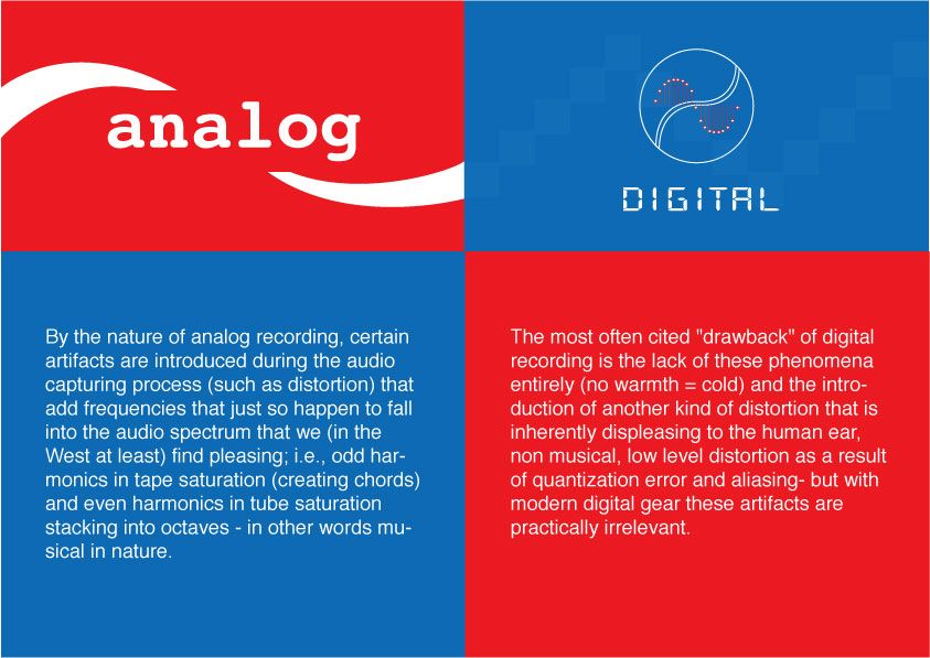
The traditional analog representation of signals is based on the similarity (similarity) of electrical signals (changes in current and voltage) with the original signals represented by them (sound pressure, temperature, speed, etc.).

Analog vs Digital

As well as in the similarity of the forms of the electrical signals in various points of the amplification or transmission path. The shape of the electrical curve that describes (also called transfer) the original signal is as close as possible to the shape of the curve of this signal.

Such a representation is the most accurate, however, the slightest distortion of the shape of the electrical carrier signal will inevitably involve the same distortion of the shape and signal of the carrier. In terms of information theory, the amount of information in the carrier signal is exactly equal to the amount of information in the original signal, and the electrical representation does not contain redundancy that could protect the carried signal from distortion during storage, transmission. and amplification.

The digital representation of electrical signals is designed to add redundancy to avoid unwanted interference. For this, serious restrictions are imposed on the carrier electrical signal: its amplitude can take only two limit values: 0 and 1. In this case, the entire zone of possible amplitudes is divided into three zones: the lower one represents zero values, the upper , unique, and the intermediate is prohibited, inward. only interference can get in. Therefore, any interference whose amplitude is less than half the amplitude of the carrier signal does not affect the correct transmission of values 0 and 1. Interference with a higher amplitude also does not affect whether the duration of the interference pulse is significantly less than the duration of the information pulse.

The digital signal formed in this way can carry any useful information that is encoded in the form of a sequence of bits: zeros and ones; electrical and sound signals are a particular case of such information. Here, the amount of information in the digital carrier signal is much higher than in the original encoded signal, so the carrier signal has a certain redundancy with respect to the original, and any distortion of the waveform of the carrier signal, which still retains the receiver’s ability to correctly distinguish between zeros and ones, does not affect the reliability of the transmitted signal. by this information signal. However, in the case of exposure to significant interference, the shape of the signal can be distorted to such an extent that the precise transmission of the information being transferred becomes impossible: errors appear in it, which, with a simple coding method , the receiver can not only correct, but also detect. To further increase the resistance of a digital signal to interference and distortion, two types of digital redundancy coding are used: verification codes (EDC – Error Detection Code) and correction (ECC – Error Correction Code). ). Digital encoding is simply adding extra bits to the original information and / or converting the original bit string into a longer string and other structure. EDC allows you to simply detect the fact of an error: a distortion or loss of a useful one or the appearance of a false digit, but the information that is transferred in this case is also distorted; ECC allows you to immediately correct detected errors, keeping the information that is transferred unchanged.

Each type of EDC / ECC has its own capacity limit to detect and correct errors, after which undetected errors and distortions of the transferred information begin again. An increase in the volume of EDC / ECC relative to the volume of the original information generally increases the detection and correction capabilities of these codes.

Like EDC, the popular cyclic redundancy code CRC (Cyclic Redundancy Check), whose essence is the complex mixing of the initial information in the block and the formation of short binary words, whose bits have a strong cross-dependence on each bit of the block. Changing even one bit in a block causes a significant change in the CRC calculated from it, and the probability of such a bit distortion where the CRC does not change is extremely small even with short CRC words (a small percentage of the length of the block). The ECC uses the Hamming and Reed-Solomon codes, which also include EDC functions.

The information redundancy of the digital carrier signal leads to a significant expansion (by an order of magnitude or more) of the frequency band required for its successful transmission.

Digital Audio Coding

Digital Audio Coding

Digital Audio coding

Digital audio technologies are used to record, process, mass produce, and distribute sound, including the recording of songs, instrumental pieces, podcasts, sound effects, and other sounds.

Digital Audio Coding

Today’s online music distribution relies on digital recording and data compression. The availability of music as data files instead of physical objects has significantly reduced distribution costs. Before the advent of digital sound, the music industry distributed and sold music, selling physical copies in the form of records and cassettes.

Using online and digital audio distribution systems such as iTunes, companies sell digital audio files to consumers that the consumer receives over the Internet. An analog audio system converts the physical waveforms of sound into electrical representations of these waveforms using a transducer such as a microphone. The sounds are then stored on analog media, such as magnetic tape, or transmitted through analog media, such as a telephone line or radio. For playback, the process is reversed: an electrical audio signal is amplified and then converted back to physical waveforms through a speaker.

Analog audio retains its fundamental waveform characteristics when stored, converted, dubbed, and amplified. Analog audio signals are prone to noise and distortion due to the inherent characteristics of electronic circuits and related devices. Interference in a digital system does not result in an error, unless the interference is large enough to cause one character to be misinterpreted as another character or to be out of sequence.

Therefore, it is generally possible to have a completely error-free digital audio system in which there is no noise or distortion between converting to digital and converting to analog. The digital audio signal can be further encoded to correct any errors that may occur during storage or transmission of the signal. This technique, known as channel coding, is necessary for broadcast or recorded digital systems to maintain bit fidelity. Modulation from eight to fourteen is a channel code used on audio CDs. Conversion process

The life cycle of sound from its source through ADC, digital processing, DAC, and finally again as sound. A digital audio system begins with an ADC, which converts an analog signal into digital. The ADC operates at the specified sample rate and converts to a known bit resolution.

For example, CD audio has a sample rate of 44.1 kHz (44,100 samples per second) and a resolution of 16 bits for each stereo channel. Analog signals that have not yet been band-limited should be damped before conversion to avoid interpolation distortion caused by audio signals above the Nyquist frequency (half the sample rate).

The digital audio signal can be stored or transmitted. Digital audio can be stored on a CD, digital audio player, hard drive, USB flash drive, or any other digital storage device. The digital signal can be modified by digital signal processing, where effects can be filtered or applied. Frequency transform Sample rates, including increasing and decreasing the sample rate, can be used to match signals that have been encoded with a different sample rate to a common preprocessing sample rate. Audio compression methods such as MP3, Advanced Audio Coding, Ogg Vorbis, or FLAC are commonly used to reduce file size.

Digital audio can be transmitted through digital audio interfaces such as AES3 or MADI. Digital audio can be transmitted over a network using Audio over Ethernet, Audio over IP, or other standards and media transmission systems. For playback, digital audio must be converted back to an analog signal using a DAC. According to the Nyquist-Shannon Sampling Theorem, with some practical and theoretical limitations, the bandwidth-limited version of the original analog signal can be accurately reconstructed from the digital signal. –

MP3 digital audio format

MP3 digital audio format

MP3 File Format

High-quality digitized audio requires a large amount of disk space.

mp3 file

Attempts to reduce the size of files using standard archivers (RAR, GZIP, etc.) do not generate significant gains due to the specificity of the sound data. However, it is possible to achieve a fairly significant level of compression of the audio information using special methods based on the analysis of the data structure and subsequent compression with some loss.

The real possibility of sound processing comparable in quality to existing analog examples did not appear until the late 1980s.

In 1988, the International Organization for Standardization (ISO) formed the MPEG (Moving Picture Experts Group) committee, whose main task is to develop standards for the encoding of moving pictures, sound and their combination. During the ten years of its existence, the committee has developed a series of norms on this subject. As a result, summarizing the extensive research in this area, several specific formats were recommended for storing data, which are excellent in quality of results and data flow.

There are currently three video storage standards: MPEG-1, MPEG-2, and MPEG-4.

Within the first two formats, there are also formats for storing audio information: Layer-1, Layer-2 and Layer-3. These three audio formats are defined for MPEG-1 and minor extensions are used in MPEG-2. The three formats are similar to each other, but use different levels of trade-off between compression and complexity.

Layer-1 is the simplest, it does not require significant compression costs, but it also provides a negligible compression ratio.

Layer-3 is the most time consuming and provides the best compression. Recently, this format has gained immense popularity. It is often called MP3. This name is associated with the extension of the audio files stored in this format.

The underlying idea behind all lossy audio compression techniques is to neglect the subtle details of the original sound that are beyond the reach of the human ear. Here several points can be highlighted.

Noise level . Sound compression is based on a simple fact: if a person is near a loud siren, they are unlikely to hear the conversation of the people who are nearby. And this happens not because a person pays close attention to a loud sound, but to a greater extent because the human ear actually misses out sounds that are in the same frequency range as a louder sound. This effect is called masking, it changes with the difference in volume and frequency of the sound.

The second point is the division of the audio frequency band into subbands, each of which is further processed separately. The encoding program extracts the loudest sounds in each band and uses this information to determine an acceptable noise level for that band. The best encoding programs also take into account the influence of adjacent bands. A very loud sound in one band can affect the masking effect and nearby bands.

Another point of the codification is the use of a psychoacoustic model based on the peculiarities of the human perception of sound. The compression used by this model is based on removing frequencies known to be inaudible, while more carefully preserving sounds that can be easily heard by the human ear. Unfortunately, there can be no exact mathematical formulas here.

The human perception of sound is a complex process, not fully understood, so the choice of compression methods is based on analyzing listening and comparing compressed sounds differently by teams of experts. But here there are practically limitless possibilities in the field of improving psychoacoustic models. Most of the existing algorithms to encode the human voice are based on the high predictability of said signal; Universal MPEG compression algorithms have tried to apply this technique with variable success.

Another compression technique is the use of so-called joint stereo. It is known that the human hearing aid can only determine the direction of the mid frequencies, the high and low sound, so to speak, separately from the source. This means that these background frequencies can be encoded into a mono signal. In addition to all this, compression uses the difference in the complexity of the flows in the channels.

Digital audio compression methods

Digital audio compression methods

Audio Compression

Lossless compression

Generally speaking, the meaning of lossless compression is as follows: some pattern is found in the original data, and taking this pattern into account, a second stream is generated, uniquely describing the original. For example, to encode binary sequences with many zeros and few ones, we can use the following replacement:

00> 0
01> 10
10> 110
11> 111

In this case, sixteen bits:

00 01 00 00 11 10 00 00

will be converted to thirteen bits:

0 10 0 0 111 110 0 0

If we write a compressed string without spaces, we can still add spaces in it, which means restoring the original sequence.

FLAC (Free Lossless Audio Codec – Free Lossless Audio Codec)
Coding principle: the algorithm tries to describe the signal with this function so that the result obtained after subtracting it from the original (called difference, remainder, error) can be encoded with the minimum of bits.

When the model is fitted, the algorithm subtracts the approximation from the original to obtain a residual signal (error), which is then losslessly encoded.

Lossy compression (MP3, AAC, WMA, OGG)
Using a lossy compression algorithm, the size of an MP3 file with an average bit rate of 128 kbps is approximately 1/11 of the original file of an Audio CD (uncompressed audio in CD-Audio format has a rate 1411.2 kbps bit rate). MP3 files can be created at high or low bit rates, which affects the quality of the result.

The principle of compression is to reduce the precision of some parts of the sound flow, which is almost indistinguishable for most people. The audio signal is divided into segments of equal length, each of which, after processing, is packed into its own frame (frame). Spectral decomposition requires continuity of the input signal; therefore, the previous and next tables are also used for calculations. The audio signal contains harmonics with a lower amplitude and harmonics that are close to the strongest; Such harmonics are cut off, as the average human ear will not always be able to determine the presence or absence of such harmonics. This characteristic of hearing is called the masking effect. It is also possible to replace two or more close peaks with an averaged one (which, as a rule, leads to sound distortion). The cutoff criterion is determined by the outflow requirement. Since the entire spectrum is relevant, the high frequency harmonics are not cut off, but are only selectively removed to reduce information flow due to rarefaction of the spectrum. After spectral removal, mathematical compression and frame packing methods are applied.

Masking effect
In certain cases, a sound can be hidden by another sound. For example, talking next to a train track can be completely impossible if a train passes. This type of effect is called masking. A weak sound is said to be masked if it becomes indistinguishable in the presence of a louder sound.

Simultaneous masking
Any two sounds, when heard simultaneously, have an impact on the perception of the relative volume between them. A louder sound reduces the perception of a weaker one, until the disappearance of your hearing. The closer the frequency of the masked sound is to the frequency of the masker, the more it will be hidden. The masking effect is not the same when the masked sound is shifted down or up in frequency relative to masking. Low-frequency sound masks high-frequency sound. However, it is important to note that high-frequency sounds cannot mask low-frequency sounds.

Time masking
This phenomenon is similar to frequency masking, but time masking occurs here. When the masking sound is stopped, the masking remains inaudible for some time. Under normal conditions, the effect of temporary masking lasts much less. The masking time depends on the frequency and amplitude of the signal and can be up to 100 ms.
In the case where the masking tone appears later than the masking, the effect is called post-masking. When the masking tone appears before the masking (this is also possible), the effect is called premasking.

Post-stimulus fatigue
Often, after exposure to loud, high-intensity sounds, a person’s hearing sensitivity drops dramatically. Recovery of normal thresholds can take up to 16 hours. This process is called “temporary change in hearing threshold.”