Audio and video Archives - Page 123 of 196

From analog to digital and vice versa

Free Download Mp4Gain

From analog to digital and vice versa

Today, almost 99% of sound recording, sound reproduction studio equipment, and music synthesizers are digital devices.

Everyone knows that even a typical home CD player uses a digital-to-analog converter and that music on CDs is written in 16-bit numbers. However, both the original sound and musical material (voice, classical musical instruments, electric guitars, etc.) and the sound output of your music center are analog signals, not digital signals. Therefore, for today’s recording industry, the key is to convert analog signals to digital and convert digital data to analog audio signals. Let’s try to find out how these transformations take place. The analog signal represents is a continuous process in time and amplitude, and its digital representation is a sequence or series of numbers that consists of a finite number of bits. The conversion of an analog signal to digital consists of two stages: time sampling and amplitude quantization. Time sampling means that the signal is represented by a series of its samples taken at regular intervals. For example, when we say that the sample rate is 44.1 kHz, it means that the signal is measured 44100 times per second. The main problem in the first stage of converting an analog to digital signal (digitization) is choosing the sampling frequency of the analog process. The answer is given by the well-known Nyquist theorem, which states that for an analog signal (continuous in time) occupying the frequency range 0 Hz to F Hz to be reconstructed with absolute precision from its samples, the frequency of The sample rate must be at least twice the maximum audio frequency F. Therefore, if the actual analog signal that we are going to convert to digital format contains frequency components from 0 Hz to 20 kHz, then the sampling frequency of that signal it should not be less than 40 kHz. Let’s take a closer look at what happens to an analog signal and its spectrum when sampled.

During sampling, the frequency spectrum changes significantly. The original analog signal tends to have a spectrum mainly concentrated in the frequency band from 20 Hz to about 20 kHz, since the usual pickups and microphones from which it is taken have about this frequency response. In addition, the signal often contains interference with frequencies of up to several hundred kilohertz. These are various “vans” difficult to remove from computer equipment, industrial and electrical appliances, trams, trolleybuses, etc. After sampling, the signal is a sequential time series of very narrow pulses with different amplitudes and with a very wide spectrum of up to several megahertz (a mathematical fact: the narrower the pulse, the broader its spectrum). Therefore, in general, the spectrum of such a pulse sequence expands to the same several megahertz. Therefore, the spectrum of the sampled signal is much broader than the spectrum of the original analog signal. Let’s take a closer look at how this new broad spectrum is set up. There are two important processes. First, the “convolution” of the entire original spectrum of the analog signal extending from approximately 20 Hz to several hundred kilohertz within the frequency band from 0 Hz to half the sampling frequency.

Convolution means that all components of the original analog signal, with frequencies above half the sample rate (and this is mostly inaudible noise)) fall in the frequency range audible to the human ear from 20 Hz to ” Average sampling frequency “Hz, ie Inaudible interference becomes audible and therefore the signal-to-noise ratio may deteriorate. All of this seems very unusual, not to say that it even contradicts common sense! It turns out that there is a sampling of high-frequency signals with frequency components that are significantly higher than not just half the sample rate, but also the sample rate itself. At first glance, this even contradicts the Nyquist theorem mentioned above. But let’s look at Fig. 4. It shows the process of sampling a high-frequency sinusoidal signal at more than two times less than its sampling frequency.

Free Download Mp4Gain

Mp4Gain Main Window

Mp4Gain Features

Free Download Mp4Gain

Psychoacoustics – highlights

Psychoacoustics – highlights

Psychoacoustics

Psychoacoustics deals with the study of the mechanisms of perception of auditory information and its interpretation by the human brain.

psychacoustic

The results obtained in the framework of various studies in this area served as the basis for the development of numerous technologies that have changed our lives in many ways. Among the most striking examples are several audio codecs, such as the well-known MP3. Internet telephony (Skype) and even mobile communications also owe their wide dissemination to research in the field of psychoacoustics.

DF Mechanism
To locate sound sources in space, using exclusively the auditory system, the human brain applies several basic principles that provide it with enough information to draw certain conclusions and make a certain decision. The main condition for this is the presence of two separate discrete receivers, which are the listener’s ears.

mechanisms of psychoacoustics

To more clearly illustrate how this works, imagine a situation where the sound source is to the left of the listener.

Time factor – ITD (interaural time difference)
The acoustic signal from the sound source will reach the right ear somewhat later than the left, since the latter is closer to the sound source. This distance (12-17 cm, depending on the size of the head) is sufficient for the brain to record the resulting time delay between two discrete receptors.

Intensity factor – IID (Interaural Intensity Difference)
The sound pressure directly on the eardrum of the left and right ear is slightly different, depending on which is closer to the sound source. The sound pressure at the eardrum of the left ear will be slightly higher than that of the right. This difference indicates the direction of the sound source.

Spectral factor
The spectral component of the acoustic signal reaching the left and right ears also differs depending on the location of the sound source. Especially high frequencies, due to the short wavelength, are shaded by the head and lose energy. In situation A, the acoustic signal reaching the listener’s right ear will contain slightly less energy in the high frequency range than that reaching the left.

The combination of the above principles allows us to orient ourselves in the ear space and plays an important role in the ability to locate sound sources in space. Every time we hear something, our brain involuntarily performs an analysis and we easily and without even thinking determine the direction from which the sound is coming.

For more information on this topic, I recommend watching the YourSoundPath video series dedicated specifically to this topic.

The mechanism for determining the distance from the sound source and the characteristics of the room.
To determine the distance from the sound source, the auditory system uses other methods. The main thing here is to determine the relationship between the fraction of the direct signal energy and the fraction of the reflected energy. The more reflections that reach the listener’s ears in the acoustic signal, the further away the sound source is. In this case, when reaching a certain radius, beyond which the ratio of reflections prevails over the energy of the direct signal, this method is no longer effective.

By analyzing the time interval between the direct signal and its reflections, the brain can draw conclusions about the distance from a reflective surface, for example, a wall, and its acoustic properties, for example, the material (concrete, glass, carpet) and the surface structure (smooth, non-uniform), etc. This is also facilitated by spectral analysis of the reflections and their density. The more diffuse they are, the more heterogeneous should be the reflective surface from which they are reflected.

Audio codecs

Audio codecs

Audio Codec

Codecs played at the same time, if not a key, a very important role in the development of technologies in the field of digital sound.

Audio Codecs

The rapid spread of mobile communications, Internet telephony, portable players – these are all examples of the use of codecs. It was only thanks to its invention and implementation that it was possible to transmit audio information through channels that were then very limited in bandwidth. This problem could be solved by increasing the capacity of all transmission channels, which would mean an incredible material investment associated with the remodeling and replacement of most of the elements of the existing infrastructure, or by developing an algorithm that can significantly reduce the amount of data. resulting from the analog to digital conversion and thus be able to use the existing infrastructure. The second way was much more sensible.

What are codecs?
A codec is an algorithm based, as a rule, on one or another psychoacoustic model, which will be discussed below, and includes two modules: an encoder and a decoder.

The encoder encodes digital audio into a data stream, the volume of which, compared to the original volume of the raw material, is significantly lower. Depending on the codec used and the encoding parameters, it is possible to achieve an optimal balance between sound quality and the desired data volume.

However, to reproduce the sound encoded in this way, a decoder is required, whose task is to decode the digital audio stream back to the standard format (PCM).

Codecs and their families
In general, all codecs, of which there are very many at the moment, can be divided into two categories:

At a loss
As mentioned above, basically the codecs work based on one or another psychoacoustic model that determines which audio information is not key for our brain and could be sacrificed and discarded, thus reducing the amount of data. The disadvantage of this method is that when decoding said transmission, the lost audio information cannot be recovered. The compression ratio can reach up to 90% of the original data volume, while maintaining satisfactory sound quality for most normal users. The most prominent representatives of this family are the well-known and perhaps the most common MP3 and WMA.

No loss
In this case, the encoding occurs without data loss, allowing all the information in the original audio signal to be fully recovered after the decoding process. However, the degree of data compression that can be achieved with these codecs is much lower than that of the Lossy family of codecs. In general, depending on the encoding parameters, compression of up to 60% of the original volume is possible. The most popular among the Lossless family codecs are FLAC, APE, and Apple Lossless on the Apple platform.

It should be noted that the vast majority of video formats also contain compressed video and audio. Formats like Dolby Digital, DTS, and their varieties are nothing more than codecs. Without a suitable decoder, it is not possible to read the audio data. In this case, maximum white noise sounds. Therefore, you must be careful not to damage your own ears and equipment.

Encoding options
The encoding parameters determine the quality of the resulting sound and the amount of data in the resulting file. More aggressive compression will reduce the sound quality and reduce the amount of data, that is, increase the compression ratio. Depending on the algorithm used, the result, or rather the quality of your sound, can differ significantly, even when using the same encoding parameters.

One of the most important is considered to be the data flow rate per unit of time: kbps (kilobits per second, the number of kilobits per second). The higher this parameter, the less aggressive the data compression will be. As a general rule of thumb, for Lossy family codecs, optimal values are 192 to 320 kbps. When lower values are used, the loss of quality becomes more significant and is noticed even by ordinary users who do not have any special rights to sound quality.

Psychoacoustic codecs and models
The vast majority of audio codecs are based on psychoacoustic algorithms that utilize the limitations of the human auditory system. These principles are based on research in the field of psychoacoustics, the most significant conclusions of which include the masking effect.

Basics of digital sound theory Part 4

Basics of digital sound theory Part 4

Sample Rate

The MP3 algorithm allows you to compress the sound 20 to 30 times while maintaining good quality.

Sample Rate

The full quality of the CD is believed to be preserved at a bit rate of approximately 160 Kbps (the concepts of “sample rate” and “sample bit depth” do not apply to MP3 files). However, in most cases, much more compressed audio is quite acceptable. Therefore, in Flash animations, MP3 compression is usually used, which gives a bit rate of the order of 16-32 Kbps. The Flash player supports a range of bit rates ranging from 16 to 160 Kbps. You must select the most suitable based on film size and sound quality requirements. It is often worth leaving the MP3 file at the same quality as imported (therefore, the Use imported mp3 quality setting is on by default). If the quality changes, then the change should be in the direction of decreasing quality, but not increasing.

If the sound is processed in an external editor, you can take into account the fact that the Flash player supports not only the MP3 algorithm, which is part of the MPEG1 Layer 3 standard, but also newer algorithms (MPEG2 and MPEG2.5), that provide better sound quality when bit depth is low. In addition, the player supports MP3 encoding with both constant and variable bit depth (in the latter case, the best compression ratio is achieved).

The MP3 format is optimal for rash projects. Therefore, in practice, it is practically only used. Furthermore, MP3 files can be loaded dynamically, and they also have very useful ID3 tags with information about this sound.

• Nellymoser. A relatively new compression algorithm developed by Nellymoser Inc. Designed to compress human speech. His main idea is that a human voice can include vibrations with frequencies in a fairly narrow range. The upper and lower components can be discarded. Very low amplitude harmonics are also eliminated. The result is compression comparable to MP3 compression, but the sound quality is higher. More details about the Nellymoser algorithm can be found on the developer’s website http://www.nellymoser.com/.

The Nellymoser algorithm codec is included in the player only in Flash MX.

In the Flash IDE, Nellymoser compression is called Speech. You can adjust the quality / size ratio when using Nellymoser compression by changing the sample rate.

You can also include uncompressed audio in your SWF movie. In the development environment, this mode is called Raw. In this case, you can change the bit depth and sample rate. In theory, you can use uncompressed audio if sound quality is significantly more important than movie size (or, even less likely, if you need to save computing resources). In practice, however, it is better to use MP3 compression with a high bit rate (more than 120 Kbps).

Storage formats
There are quite a few audio formats. By default, Flash only allows you to import two of them.

• WAV. The main format for storing uncompressed audio on the Windows platform. Supports mono and stereo audio, various samples, and bit depths. Usually it is WAV where the analog signal is digitized, and only then is one of the compression algorithms applied. WAV files are extremely large, which is why this format has been significantly replaced by MP3. However, WAV is still the main format for professional sound editors like SoundForge.

• MP3. Audio format using the compression algorithm described above. The main format in the case of Flash, as it perfectly combines good sound quality and a small file size. Also, sound files in this format, unlike WAV files, can be dynamically loaded into a movie using the loadSound () method of the Sound class.

If you have QuickTime 4 or higher installed, you can import files in AIFF, QuickTime, Sun AU formats additionally.

Basics of digital sound theory Part 3

Basics of digital sound theory Part 3

Sample Rate

Compression algorithms

Sample Rate

Let’s try to calculate how much disk space an average CD-quality digitized music composition will occupy. Obviously, for this it is necessary to use the formula t KBF size ⋅ ⋅ ⋅ = where F is the sampling frequency, B is the sample capacity, K is the number of strings, t is the time.

Assuming 44.1 kHz herbal, B = 2 bytes, K = 2 channels, and t = 300 seconds, we get that the digitized song will occupy approximately 50MB.

This means that only about 10 uncompressed songs can be burned to CD. Since every second of digitized CD quality sound takes up almost 200 Kb, this sound will be very problematic to use on telephony, radio or the Internet. Even if you digitize the sound as a single channel with a sample rate of 11.05 kHz and a bit depth of 8 bits, each second will occupy 11 KB.

For ordinary telephone networks, this is too much for sound to be transmitted in a continuous stream. A problem arises: somehow it is necessary to reduce the size of the sound files.

It is solved quite effectively by using various compression algorithms.
Flash Player supports the following types of compression.

• ADPCM (Adaptive Differential Pulse Code Modulation – Adaptive Difference Pulse Code Modulation). This type of compression is based on two ideas. First, it was found that in the vast majority of sounds we perceive, slowly changing low-frequency components prevail. From this fact it follows that the difference between adjacent samples is often small (or rather, significantly less than the absolute value of the samples themselves).

This means that the digitized audio signal can be represented not by the samples themselves, but by the differences between them, which are smaller in magnitude and therefore require fewer bits for description. Second, the coding of the difference between adjacent samples is done taking into account the magnitude of the amplitude and frequency composition, since the human ear has sensitivity limits (the so-called adaptation).

The ADPCM algorithm is actively used in IP telephony. It is poorly suited for streaming music due to the significant distortions it introduces into sound (distortions, of course, get into speech, but are hardly noticeable in speech). The compression ratio for ADPCM is typically low, ranging from 8: 1 to 3: 1. The ADPCM Flash Player codec allows 2, 3.4, or 5 bits to represent the difference between samples. Actually, you can achieve acceptable sound quality with a bit rate (bit rate, that is, the “weight” of a second of sound) of 16 Kbit.

The ADPCM algorithm is significantly inferior to MP3, so it is not worth using such compression in principle. MP3 compression will provide an order of magnitude better quality with the same bit depth. The presence of the corresponding codec is explained by the principles of backward compatibility: the MP3 codec is built into the player only in Flash 4. Before that, only the ADPCM codec was used, which is probably due to the free distribution of this algorithm. The reason ADPCM is still used in IP telephony is that it does not require as extensive math calculations as MP3, so compression can be done on the fly.

• MP3. One of the first and most common compression algorithms based on the so-called psychoacoustic compression. It uses the following characteristics of the human ear:

or if a soft sound follows a very strong one, then we don’t hear it. Therefore, it can be discarded;

or a sound component with a large amplitude masks components close to it in frequency, but with smaller amplitudes. Therefore, they can be slaughtered without noticeable loss of quality;

or the ear’s sensitivity to frequency distortion is low, therefore, if the components are close, they can be considered the same;

o We misperceive very low and very loud sounds, so fewer bits can be allocated for their encoding than for sounds with an average frequency.

Technically, the MP3 algorithm is implemented as follows. The sound is divided into chunks of a certain length called frames, and a forward Fourier transform is applied to each set of samples. Its result is the decomposition of a sound wave into elementary sinusoids of different frequencies: harmonics. The harmonic coefficient determines its contribution to the resulting wave. Harmonic coefficients are compared and the least significant are discarded.

Basics of Digital Sound Theory Part 2

Basics of Digital Sound Theory Part 2

Sample rate

A sample rate of 44.1 kHz is not always ideal.

Samplerate

When transmitting data over a low-bandwidth network, the quality of the sound must be sacrificed in favor of its size, in practice sampling frequencies two, four and eight times lower than 44.1 kHz are usually used:

• 22.05 kHz: the so-called radio quality. Used when encoding the sound of FM radio stations. In the case of Flash, it is good for creating background music and event sounds. For the transmission of a human voice, it is even somewhat redundant;

• 11.025 kHz – telephone quality. A sample rate more suitable for the human voice. Used in 1P telephony;

• 5.5 kHz: sound about to lose the information component. This sample rate can be used to transmit low sounds as well as speech (albeit with mediocre quality).

Flash Player supports sample rates 44.1: 22.05; 11,025; 5.5 kHz. The choice of frequency should be determined by the type of sound, as well as the importance of maintaining the size of the SWF file. However, it should be remembered that there is no point in increasing the sample rate of the audio fragment compared to the initial one. This will not increase the quality, but will only unnecessarily increase the size of the movie.

Bit depth of samples
Bit depth determines how many different amplitude values can be captured during digitizing. If the bit width is 4 bits, then the range of the amplitude value from zero to the maximum will be divided into only 16 bins. Naturally, the error when rebuilding the analog signal will be very high. This bit depth is suitable for representing very simple sounds as well as speech (its quality will be low).

The 8-bit width allows 256 amplitude values to be represented. This is the bit depth used by FM radio stations. It is enough to present any sound in satisfactory quality. 16-bit encoding is optimal. At the same time, it can work with 65,536 amplitude options, which is enough to cover the entire audible range.

The 16-bit format is used for CD recording. Higher quality quantization is only justified in the case of studio sound processing.

Flash Player supports 8-bit and 16-bit quantization for uncompressed formats (for example, WAV) and only 16-bit for compressed formats (MP3 belongs to them). Keep this in mind when importing a sound file into a movie.

Number of channels The
Stereo sound is designed to give the playback sound a natural dimension. This is achieved due to the fact that a different component of sound is reproduced from each speaker. In general, the sound of each channel is a separate sound file, so the size of the stereo sound is proportional to the number of channels supported.

Conventional non-professional sound cards work with two-channel audio. The Flash player also supports the same number of channels. With ActionScript, you can mix the sound of the channels by playing the left channel on the right speaker and the right channel on the left. How this is done, we will talk a bit below.

If the sound is encoded in MP3 format, you can choose one of three stereo formats.

• Dual channel. Each channel receives half of the stream and is separately encoded as mono. It is mainly recommended in cases where different channels contain a fundamentally different signal, for example text in different languages.

• Stereo. The channels are scrambled separately, but the scrambler program can give one channel more space than the other if necessary. Most standard format.

• Joint stereo. The stereo signal is divided into two new channels. One is the average of the original channels and the other is the difference between the channels. In this mode, the sound quality is obtained more frequently than in others.

Unfortunately, in the Flash development environment, you cannot specify which stereo format is used. Therefore, if sound quality is of paramount importance, then the creation of MP3 files with the required parameters should be done using one of the specialized programs.

Basic concepts of digital sound theory

Basic concepts of digital sound theory

Sample Rate

Sound is, in general, the vibrations of an elastic medium.

sample rate

The sound is caused by mechanical vibrations of some object (this can be a string, vocal cords, etc.) in contact with the environment. The frequency of vibration (measured in Hertz) determines the pitch. The higher the frequency, the louder the sound. The human ear can perceive sound vibrations from the air with a frequency of 20 Hz to 20 kHz. The ear perceives the amplitude of the vibration as volume. The higher the amplitude, the louder the sound.

Electromagnetic waves are a direct analog of sound waves. The latter are less susceptible to dispersal by the environment, the information they carry is easier to store and process. Electromagnetic waves are the most important secondary carrier of sound. The transformation of acoustic waves into electromagnetic waves (as well as the reverse operation) is carried out due to the usual induction effect, which consists in the appearance of a current in a conductor when it is placed in an alternating magnetic field.

Simply put, the oscillation of the loudspeaker membrane magnet near the coil induces an alternating current in it. If this current is applied to another speaker, then the magnet on its membrane will move, creating a corresponding sound.

This is how the telephone and the radio work.

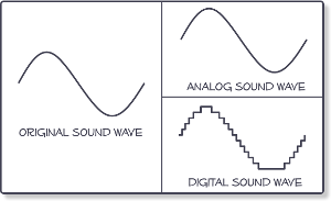
Sound converted to electromagnetic waves can be easily stored. For this, some parameter of the carrier must be compared (the depth of the plate track or the degree of magnetization of the film) with the amplitude of the oscillations (that is, the strength of the induced current in the speaker coil) . Sound converted directly to electromagnetic waves is called analog sound. Its main characteristic is the direct correspondence of the electromagnetic waves transmitted or recorded with the acoustic ones.

Digital sound is relatively new. Its main difference from analog is discretion. When digitizing, a special device, an analog-to-digital converter (ADC), measures at regular intervals (approximately 0.001-0.0001 seconds) the magnitude of the amplitude of an electromagnetic wave corresponding to an analog sound form and writes its value to a file with a specified precision. This value is generally called sample, or in jargon, sample (of the sample in English, sample). The same digitization is often called sampling or sampling.

By converting sound from digital to analog (this is done by a device called a digital-to-analog converter (DAC)).

The interpolation (approximation) of the intermediate values of the amplitude is carried out according to the known ones. Since the sampling frequency is usually high, this operation allows you to fairly accurately reconstruct the original analog signal.

The digital form of sound is characterized by five parameters.

1. The sampling rate;
2. Bit size of the samples.
3. The number of channels or tracks.
4. Compression / decompression algorithm (codec).
5. Storage format.

Since each of these parameters is quite specific, we will consider them separately.

Sampling rate
The sample rate determines how many samples per second will be taken when digitizing. If we compare digital sound with digital images, then the sample rate will correspond to the resolution (a more “realistic” analogy is the frame rate in cinema). The higher the sampling frequency, the better it is possible to reconstruct the analog signal based on the digital form of the sound (more precisely, the higher the sampling frequency, the broader the spectrum of frequencies that can be recorded during digitization).
The famous Nyquist-Kotelnikov theorem states that for the correct reconstruction of an analog signal from its digital recording, it is necessary that the sampling frequency be at least twice the maximum sound frequency.

Since the upper listening limit is 20 kHz, ideally the sample rate should be at least 40 kHz. This is why the standard sampling frequency used for recording CDs is 44.1 kHz (so-called CD quality). However, the sample rate can be higher, but this sound quality is only used by recording studios and especially demanding music lovers.

Sample rate and bit depth

Sample rate and bit depth

uno

When describing digital recording devices, two fundamental concepts are used: sample rate and bit depth. In this article, we will see what it is.

Sampling rate
The sample rate is the rate at which the logger captures samples of the input signal. When recording sound in digital form, in fact, individual samples or, in other words, values of sound intensity are recorded at separate points in time.

The sample rate for recording devices is usually the following standard values: 44.1 kHz; 48 kHz and 96 kHz. The higher the sample rate, the more samples will be taken in 1 second and the better the digital sound quality we will get as a result.

What is the meaning of these numbers? They mean the number of times the recorder reads the sound intensity value from the input signal per second. The sample rate is measured in kilohertz (kHz), 1 kHz = 1000 samples per second.

For example, if the recording is made with a sampling frequency of 48 kHz, this means that the sound recorder measures and records the sound intensity value 48,000 times per second.

This number may seem unimaginably huge, but here the phenomenon called Nyquist frequency is worth remembering. The Nyquist frequency is named after the person who first discovered it. Defines the highest sound frequency that can be recorded at a given sample rate.

In short, the maximum tone that can be digitally fed is about half the sample rate.

Therefore, when recording at a sampling frequency of 48 kHz, the maximum audio frequency that can be recorded is 24 kHz. This is sufficient, considering that the human ear hears frequencies on average from 20 Hz to 20 kHz.

Bit depth
When talking about digital recording devices, you can often hear the words “16-bit”, “24-bit”, and so on. Some mean the number of information units with which the value of each sample obtained from the digital recording can be represented.

The higher the value of this number, the more accurately you can record the value of each sample and the higher the sound quality you will get as a result.

Do not think that the greater the number of bits, that is, the greater the bit depth, the greater the intensity value that can be set. Here is meant representation precision.

Modern recorders are usually 24 bits wide. It should be noted that recording with a large bit depth takes up a lot of space on the storage device, but this is not so important, because modern media has a huge volume and is becoming more and more affordable.

Why upsampling? Part 1

Why upsampling? Part 1

Upsamplin

When it comes to improving digital sound quality, experts in this field agree on only one thing: As the sample rate increases, the sound quality improves dramatically.

Upsampling

Also, under the word “improve”, everyone already understands something of their own. All the variety of opinions on this topic boils down to the following: the sound becomes clearer, softer, more natural, the low frequencies are perceived more clearly.

However, these nuances are only noticed by listeners trained with a good ear for music on specially selected sound material and using technically advanced equipment.

There are many hypotheses that explain why sound quality is improved by sampling. Many technicians are inclined to believe that this relationship is due to distortions that arise from filtering and interpolation during reconstruction of the audio signal.

On a modern technical level, high-quality interpolators may be practically impossible to implement, therefore instead of improving them, manufacturers simply increase the sampling rate. Maybe it’s not about them at all.

Another version, which many music lovers adhere to, is that at a low sampling frequency, for example 44100 Hz, digital sound is completely devoid of nuances of high sounds, the main frequencies of which are above 7 kHz. , and at lower frequencies there are too few nuances for high quality. perception of music.

In fact, many musical instruments generate vibrations of up to 100 kHz. It is true that the proportion of energy that falls in the frequency band above 20 kHz is 0.01 to 2% for sounds of a harmonic nature and 0.02 to 68% for sounds created by a cymbal, triangle or hitting a drum rim. metal (hoop shot – Editor’s note).

Even the frequency range of speech in hissing-hissing sounds extends up to 40 kHz. Supporters of this version are not ashamed that a person cannot perceive sounds with a frequency higher than 20 kHz. Ultrasound is assumed to be perceived bypassing the auditory system, for example, through bone conduction.

Rumors that harmonics above 20 kHz contribute significantly to sounding have led to the creation and widespread introduction of analog-to-digital converters using 96 kHz and 192 kHz sample rates; The sampling frequency is expected to increase to 384 kHz.

Based on modern knowledge of human perception of sound, it must be assumed that the relationship between digital sound quality and sampling frequency is due to the transformation of the quantization error spectrum in the audio frequency range.

In the technical literature, this topic is considered only for a particular mathematical model, when music is represented by a signal with a uniform distribution in level and frequency. In this case, the quantization errors are converted to noise with a uniform spectral density from 0 Hz to the Nyquist frequency.

For every doubling of the sampling frequency, the spectral noise density is reduced by half and the signal-to-noise ratio increases by 3 dB. Since the pressure resolution limit is approximately 1 dB, these decibels are unlikely to have a noticeable effect on sound perception in the high-frequency region. Based on these numbers, it is absolutely impossible to draw tentative conclusions about the change in sound quality.

In order to relate the spectrum of quantization errors, sampling frequency and sound quality, in this article it is proposed to use a tonal signal as a music model, as is usual to evaluate the quality of sound paths. This approach is largely based on materials published in the “Sound Engineer” magazine.

The results can be summarized as follows. Unlike analog audio, digital audio is the product of amplitude modulation. This is manifested in a rigid functional dependence of the frequency multiplicity factor quantization error spectrum of the audio signal frequency F and the sampling frequency fs, represented as the ratio of the prime numbers y and x (k = fs / F = y / x). The frequency spectrum of quantization errors is always discrete and is uniquely determined by the multiplicity factor; the components of this spectrum are also uniquely determined by the amplitude of the audio signal, expressed in quanta. This means that the mechanism for the formation of the quantization error spectrum does not depend on the number of bits used. With an increase in quantization bit depth.

24/192 digital audio format and why it doesn’t make sense. Part 4

24/192 digital audio format and why it doesn’t make sense. Part 4

Oversampling

Misunderstand the sampling process

Sampling theory is often incomprehensible without the context of signal processing. And it’s no wonder that most people, even brilliant doctors in other fields, don’t get it. It’s also not surprising that many people don’t even realize that they are making a mistake.

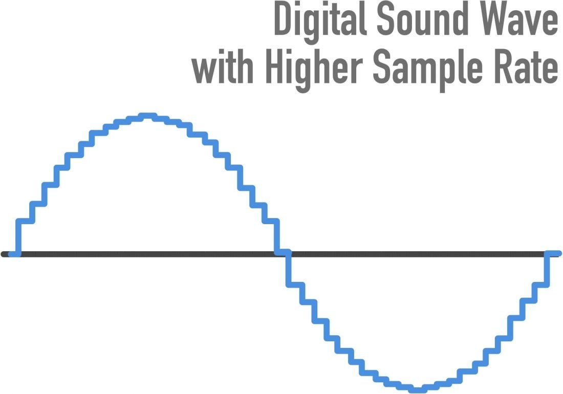
The sampled signals are often represented as a serrated ladder, as in the figure above (in red), which appears to be a rough approximation of the original signal. However, this representation is mathematically accurate, and when converted to an analog signal, its graph becomes smooth (blue line in the figure).

The most common misconception is that sampling is a crude process and leads to loss of information. The discrete signal is often represented as a jagged, angular stepped replica of the original perfectly smooth waveform. If you think so, you can assume that the higher the sample rate (and more bits per sample), the smaller the steps and the more accurate the approximation. The digital signal will look more and more like analog form until it takes shape at a sample rate close to infinity.

Similarly, many people who process non-digital signals will look at the image below and say, “Ugh!” It may appear that the discrete signal does not represent the high frequencies of the analog waveform well, or in other words, as the frequency of the sound increases, the sampling quality drops and the frequency response degrades or becomes sensitive to the phase of the input signal.

It just looks like this. These beliefs are wrong!

All signals below the Nyquist frequency (half the sample rate) will be captured perfectly and completely during sampling, and an infinitely high sample rate is not needed for this. Sampling does not affect frequency response or phase. The analog signal can be recovered without loss, as smooth and synchronous as the original.

You can’t argue with the math, but what are the difficulties? The best known is the bandwidth limitation requirement. Signals above the Nyquist frequency should be filtered before sampling to avoid alias distortion. The infamous anti-aliasing filter acts like this filter. The suppression of sampling noise, in practice, may not be perfect, but modern technologies allow you to get very close to the ideal result. And we come to oversampling.

Oversampling

Sample rates above 48 kHz are not relevant for high fidelity audio, but are necessary for some modern technologies. Oversampling (oversampling) is the most significant of them [7].

The idea of oversampling is simple and elegant. You may remember my video “Digital Media. A Guide for Beginner Geeks ”that the high sample rates provide a much larger gap between the highest frequency that we care about (20 kHz) and the Nyquist frequency (half the sample rate). This enables simpler and more robust anti-aliasing filters and improves fidelity. This extra space between 20 kHz and the Nyquist frequency is essentially a buffer for the analog filter.

The figure above shows diagrams from the video “Digital Media. A beginner’s guide illustrating the transition bandwidth for a DAC or ADC at 48 kHz (left) and 96 kHz (right).

This is only half the battle because digital filters have fewer practical limitations than analog filters and we can complete the smoothing with greater precision and efficiency. The dry high-frequency signal passes through a digital anti-aliasing filter, which has no problem placing the filter’s transition band in tight spaces. Once the straightening is complete, the additional discrete sections in the cushioning space are simply folded back. The oversampled signal is reproduced in reverse.

This means that signals with a low sample rate (44.1 kHz or 48 kHz) may have the same fidelity, smooth response, and low aliasing as signals with a sample rate of 192 kHz or higher, but none of them will appear. . disadvantages (ultrasonic waves causing intermodulation distortion, increased file size). Almost all modern DACs and ADCs oversample at very high speeds, and few people know this because it happens automatically within the device.

DACs and ADCs have not always been able to oversample. Thirty years ago, some recording consoles used high sample rates for sound recording using only analog filters. This high frequency signal was later used to create master records.