Bitrate and its calculation Bit rate (bit rate)


Free Download Mp4Gain
picture

Bitrate and its calculation Bit rate (bit rate)

bit rate

Flow rate data per unit of time.

bit rate

Information flow is normally measured in bits and transit time in seconds (bit / s, bps). There are other quantities derived with the prefixes kilo- and mega- (kbit / s, kbit / s, kbps, Mbit / s, Mbps, Mbps). Bit rate is one of the main parameters of a video. Its value affects the size and quality of the video file. The bit rate is directly proportional to the quality and size of the file. The higher the bit rate, the better its quality and the larger the file size. Two types of speed must be distinguished: maximum bit rate: the maximum number of bits that can pass per unit of time, and bit rate: the bandwidth of the channel without delay.

Data stream compression modes

Constant Bit Rate Constant Bit Rate (CBR) is the encoding of the data stream, specified by the user and has a constant value throughout the length of the file. This mode improves compatibility and the ability to calculate more accurately, but can increase the size of the output file. Do not use this mode for dynamic scenes (sports programs, action movies, etc.) and when objects are moving in different directions. Variable Bit Rate (VBR) Variable Bit Rate is a mode in which the codec determines the amount of information stream transmitted based on the complexity of a given file segment. This mode produces the best quality in an optimal size and prevents flickering. The disadvantages of this method include only the unpredictability of the output file size and the possibility of incompatibility. Variable bit rate is actively used for burning Blu-Ray and DVD discs, where there is no limitation on the size of the file as such. Average Bit Rate (ABR) Average Bit Rate is a combination of variable and constant bit rates set by the user. Unlike variable bitrate, the data stream varies within strict limits and does not reach the minimum and maximum values. This allows you to predict the output file size much more accurately than VBR and improve video quality in fast-moving video scenes. The method was applied in the network. This mode is sometimes used to compress audio.

Bitrate calculation

Having mastered what the bit rate is and having disassembled the compression modes of the flow of information, we can proceed to the independent calculation of the bit rate. Let’s establish the conditions of the problem: video: home video 120 minutes long sound: present; menu: necessary; DVD-R Media (DVD + R) 4.36 GB; Output format: DVD (MPEG-2) DVD-R size: 4.36GB = 4464MB. Size is critical, so we will be calculating from 4300MB for several reasons: 1. Bitrate cannot be accurately calculated and the file may be larger than planned. All full disk space sometimes leads to improper disk startup. 3. Many programs are recoding based on this value. We subtract another 300MB for the menu and the audio track (if your sound is not in PCM format, whose bit rate is much higher, and if you don’t plan to create multiple audio tracks) and we get 4000MB. 4000: (120 * 60) = 0.556 Mbps = 0.556 * 8 = 4.444 Mbps = 4.444 * 1024 = 4551 Kbps. For a high-quality DVD-Rip, this value is ideal, but for MPEG-2 it is barely supportable. The fact is, different video formats need different bitrate values ​​for an acceptable picture. You can try to play this video and if there are dynamic moments, you will see artifacts in the shape of squares in the video. It follows from this that you need to reduce the length of the file to about 60 minutes or look for other compression methods.


Free Download Mp4Gain
picture


Mp4Gain Main Window
picture


Mp4Gain Features
picture


Free Download Mp4Gain
picture

What is video encoding? Part 3

What is video encoding? Part 3

video encoding

MP 3

video encoding

MP3 (MPEG-1 Audio Layer-3) is a standard technology and format for compressing an audio stream into a very small file (reduced by approximately 20 times the size of the original file) while maintaining the same level of quality as the file original audio. . MP 3 technology uses psychoacoustic modeling to reduce the size of the audio file and maintain a high level of sound quality.

MPEG
MPEG stands for Motion Picture Expert Group and MPEG stands for the generic name for video formats. A group of experts defines standards for digital video such as MPEG -1 (used in Video CD), MPEG -2 (used in DVD and SVCD), MPEG -4 (used in DivX video technology), as well as some audio standards, among others that MP 3 and AAC.

MPEG -4
MPEG-4 is a standard developed by the 11th MPEG Working Group of ISO (International Organization for Standardization) in October 1998 (the date of the first draft of the standard). MPEG-4 is the standard for the mature digital age. With its additional features, MPEG-4 offers better compression, interactivity, and versatile wireless data / Internet access.

Multipass encoding – multipass encoding
True multi-pass encoding is currently only available for WM8 and MPEG-2 (SVCD and miniDVD). The multi-pass encoder analyzes the video stream on the first pass and writes everything it finds to log files. Let’s say we have a shortcut that starts with a dialogue scene where we cut something out and the camera remains stationary. Then we move on to karate shots, with a host of rapidly changing scenes and actively developing action (people flying in the air, kicking, punching, etc.).

Usually with a constant bit rate the encoder receives a higher or lower bit rate every second (this can only be called a constant 100% bit rate, but these are details). While in multi-pass variable bit rate mode, the encoder will use the bit rate according to the knowledge of the video stream, that is, the dialogue scene will receive a dedicated bit rate and the fight scene it will be much greater.

The more passes there are, the more perfect the bitrate distribution will be. In a single variable bit rate pass, the encoder must base its decision on where and what bit rate to use solely on knowledge of the composition of its previous encoding.

PCM
Pulse code modulation is the simplest binary representation of digital audio. The audio signal is converted into samples (samples) corresponding to the frequency of the signal. Then each sample (sample) is written in sequence, without using heavy compression techniques.

What is video encoding? Part 2

What is video encoding? Part 2

video encoding

Bit rate – bit rate

video encoding

The bit rate is the bit rate of the data transmission, that is, the number of bits transmitted per unit of time, generally measured in bits per second. When encoding video, a distinction is made between video and audio bit rate; During encoding, each parameter is set to its own value and does not depend on the other.

Shine – shine
(1) Intensity of color, measured from black (zero brightness) to white (maximum brightness).

CBR / VBR constant / variable bit rate
Constant Bit Rate / Variable Bit Rate: Constant / Variable Bit Rate. With a constant bit rate, the same number of bits is allocated for each frame of the movie. With a variable bit rate, frames that require better quality get more bits and vice versa. Note that dynamic movie scenes require more bits than smooth scenes.

Codec -codec
COder / DECoder – COder-DECoder (short codec): A codec is a piece of software that allows you to encode data (usually audio or video) in a specific format, and it can also decode data encoded in this format. Popular codecs: MPEG -1, MPEG -2, MPEG -4, Indeo, etc.

AVI, ASF and others are not codecs, but data formats that can be obtained using codecs.

Composite video – composite video
This is a signal in which luminance, chrominance, and timing are combined into a single signal used in the television broadcast standard.

Decoding – decoding
The term Decoding describes the process of converting a compressed (encoded) file into a viewable image.

Deinterlace – deinterlace (remove interlacing)
It is the process of removing artifacts caused by the nature of interlaced video (two fields per frame). Otherwise, it is called the “comb effect.”

Encoding – encoding
It is the process of compressing a “raw” uncompressed file by encoding it in a given format while maintaining a certain quality.

FilmFX
This post-processing algorithm adds “warmth” to video for those users who like warm tones rather than the clarity of digital video. The FilmFx filter is best suited not only for adding warmth to a movie, but also for reducing perceived blockage in digital video and decreasing processor load during decoding.

Frame – frame
This is the basis of the entire film, one frame represents one image. Film generally runs at 24, 25, or 30 frames per second, which is equivalent to displaying 24 (25 or 30) images per second. Imagine 24 images of one bird each. In the first image, the bird is on the left, in each subsequent image, it gradually shifts to the right, in the last image, the bird is on the right edge. When these 24 images are displayed in sequence very quickly, the human eye will see the bird flying from left to right.

Global motion compensation: general motion compensation
Global Motion Compensation (GMC) – Global Motion Compensation helps enhance complex scenes including panning and zooming. The ability to reduce the amount of data from one frame to the next may be diminished as there are some similarities between panning and zooming an image. To more effectively compensate for movement, this similarity can be exploited in the groups of blocks found most frequently in such scenes.

Keyframe – Keyframe
Full frame, but highly compressed (compressed).

What is video encoding?

What is video encoding?

video encoding

I suppose I will not be wrong to say that this is a rather delicate and complex process, fraught with many difficulties and problems.

video encoding

Well, first of all, you need to understand clearly enough for yourself that the video encoding process, in any scenario of the main and accompanying factors, always leads to an overall decrease in the quality of the video stream. But the whole question and all the excitement, so to speak, is how much will we lose in quality and whether our loss will be proportional to the size of the resulting video file. In general, we try to repackage the video in such a way that with a slight decrease in quality, we get a visible gain in size.

Now let’s move on to more “mundane” things … “It is known for sure” 🙂 that any video sequence is a sequence of images that alternate at a certain speed, the so-called FrameRate (frame rate). Each image has a set of certain parameters such as: frame size (FrameSize), color depth, brightness, contrast, etc. All these parameters are very important and leave a serious mark on the final video. Unfortunately, video quality is a subjective factor in our perception of this or that video stream, for each person the line between acceptable quality and disgusting “screen” is different. In this regard, I would like to point out that although the quality of video material is an important benchmark in the world of encoding, it unfortunately does not have strictly regulated characteristics.

Now in a nutshell, directly about the process itself …

As an example, let’s take the well-known and fairly easy-to-use DrDivX program. Let’s start our debriefing with the terminology …

AC3
Also known as Dolby Digital from Dolby LabsTM. It can support up to 5.1 channels of audio.

AVI
Audio Video Interlacing – Audio Video Interlacing (joining them together) – This is a video and video format commonly used on Windows operating system computers. This format is defined as a kind of combination of audio and video data, without specifying any specific codec.

B-frames / bidirectional encoding
There are three types of frames that are possible in a DivX video stream. These frames are called I-frames (intra), P-frames (predicted), and B-frames (bidirectional). Before the release of the DivX 5.0 codec, only I and P-frames were used. I-frames are encoded using information only from the encoded frame itself and do not use information from other frames (time compression). I-frames are based on conventional single-frame compression to the JPEG format. P (predicted) frames predict next frames and can also refer to I or P frames, that is, E. P frames are encoded using information from previous frames. In any video sequence, there will always be a group of frames, many of which will be the same and will contain the same image. For example, if you are watching news, and you pay attention to any moving character, you may notice that for several frames the background behind him almost always remains unchanged. (Remember that normally the frames are rotated at 25 or 30 frames per second). So instead of encoding each frame in JPEG format independently, you can take advantage of the redundancy of previous frames by applying P-frames. Basically, P-frames are future frames, defining how a block from a previous frame has been moved. at the current P-frame. So instead of spatially encoding the frame, the P-frame just says “Hey block, in the frame above, move to point (X, Y)”. This time encoding algorithm requires much less data than the spatial encoding of each frame. Basically we are passing the difference between adjacent frames, which is more efficient,

Bit depth

Bit depth

Bit depth

To understand bit depth (width), we first look at bits.

Bit depth

Short for binary digit, a bit is a separate component of a binary code, either 1 or 0.

The more bits used, the more possible combinations. For example …

As you can see from the table below, 16 combinations can be made from 4 bits.

4 bits

When used to encode information, each number is assigned a value.

As the number of bits increases, the number of possible values ​​grows exponentially.

4 bits = 16 possible values
8 bits = 256 possible values
16 bits = 16536 possible values
24 bits = 16777215 possible values
In digital audio, each value is assigned to the amplitudes of the sound wave.

The higher the bit depth, the greater the difference between loud and quiet sound … and the greater the dynamic range of the recording.

As a general rule of thumb, with each “beat”, the dynamic range increases by 6 dB.

For example :

4 bits = 24 dB
8 bits = 48 dB
16 bits = 96 dB
24 bits = 144 dB
In general, this means … more bit depth results in less noise …

Because by adding headroom, the desired signal can be recorded more clearly in relation to noise.

small and large drill depth

Further away…

5. Quantization error
It sounds amazing that there are almost 17 million values ​​in 24-bit recordings, right?

However, this is much less than the infinite number of possible values ​​that exist in an analog signal.

In almost all samples, the true value is somewhere between the two possible values. The converter simply rounds (quantizes) them to the nearest value.

The result is a distortion known as quantization error, which occurs in two stages of the recording process:

at first, during analog to digital conversion
at the end, during mastering
During mastering, the sample rate and bit depth of the final track are often reduced when converted to the final digital format (CD, mp3, etc.).

When this happens, some information is removed and re-quantized, further distorting the sound.

To solve this problem, the following was invented …

6. Dithering
When converting a 24-bit file to a 16-bit file, dithering is used to hide most of the resulting distortion.

Adding “pseudo-random noise” to the audio signal.

Since this concept is difficult to visualize when talking about sound, it is usually explained using pictures.

It works like this:

When a color photo is converted to black and white, it is mathematically calculated which color pixel should be black and which pixel should be white.

Also how the quantization of digital audio samples is calculated.

As you can see from the illustration below, the above image looks like shit, doesn’t it?

hesitate

But thanks to dithering …

a small amount of white pixels are accidentally inserted into the black areas …
a small number of black pixels accidentally get into the white areas …
And by adding this “pseudo-random noise” to the image, the “after” image looks much better. The concept of audio dithering is similar to this.

Further away…

7. Delay time
A MAJOR FAULT of modern digital studios is the delay that builds up in the signal flow, especially in DAWs.

Taking all the calculations into account, it takes anywhere from a few milliseconds to several millisecond TENS for the audio signal to exit the system.

The 0-11 millisecond delay is so short that the average person wouldn’t even notice it.
With a delay of 11 to 22 milliseconds, you will hear an annoying slapback, a short delay that takes some getting used to.
With a delay of more than 22 milliseconds, it is almost impossible to play or sing along with the track.
In a typical digital signal chain, there are 4 stages that affect the resulting delay time:

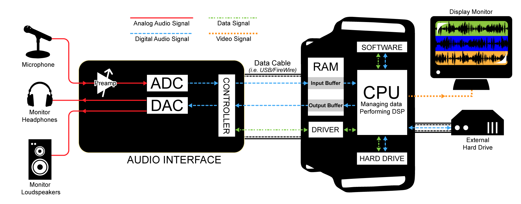
analog to digital conversion
DAW buffering
complement delay
digital to analog conversion
A / D and D / A conversion are the 2 smallest negative effects that add a maximum of 5 milliseconds to latency.

The beginning of the digital age

The beginning of the digital age

digital audio

binary code

digital audio

Although digital audio is the standard of music these days …

It has not always been this way.

Music originally existed only in the form of sound waves.

Then, with the development of technology, ways were discovered to convert it to other formats, such as:

Musical notation
electrical signals in cables
radio waves in the atmosphere
request on vinyl record
But more recently, in the age of computers, digital audio has become the main recording format, making it easy to copy and transfer songs.

The device that made this possible is called … digital converter.

Also, on how it works …

2. Digital converters
In recording studios, digital converters exist in 2 versions:

as a standalone device in top studios or …
as part of an audio interface in home studios.
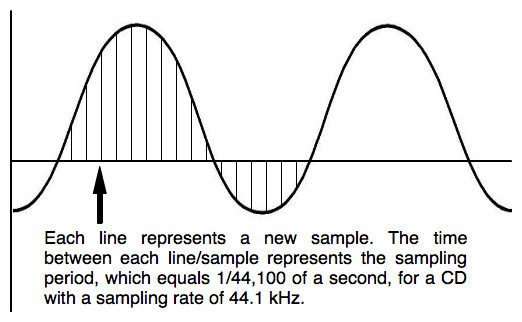
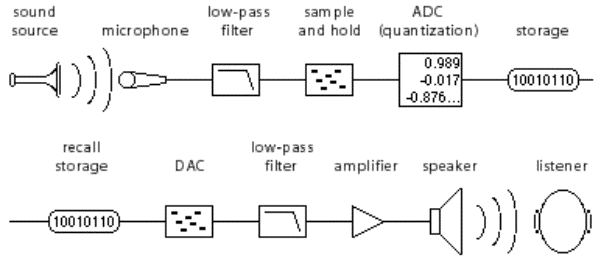
To make binary code out of sound, they take tens of thousands of images (samples) per second to build a rough image of an analog wave.

This image is not entirely accurate, because in the moments between samples, the converter has to guess what is happening.

digital wave

As seen in the graphic above:

the red line shows an analog signal and …
black line shows conversion …
The results are not ideal, but sufficient to produce excellent sound quality.

And the difference depends mainly on …

3. Sampling rate
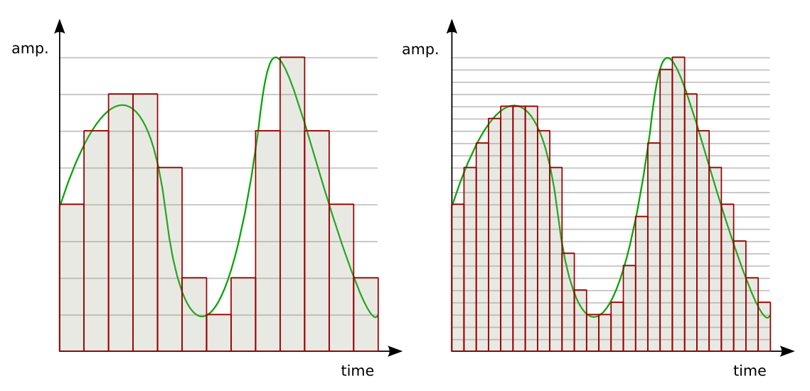
Take a look at this image:

sampling rate circuit

As can be seen …

By capturing more images per second, higher sampling rates:

Collect more real information,
Use less guesswork,
Creates a cleaner display from an analog signal
And in the end, you get the best sound quality.

Now let’s talk about specific numbers:

Standard sample rates in professional audio:

44.1 kHz (CD)
48 kHz
88.2 kHz
96 kHz
192 kHz
44.1 kHz is the minimum sample rate due to a mathematical principle known as …

Kotelnikov’s theorem (Nyquist-Shannon)
To accurately record digital audio, converters must capture the full spectrum of human hearing between 20 Hz and 20 kHz.

According to Kotelnikov’s theorem …

Capturing a specific frequency requires at least 2 samples per cycle … to measure both the high and low points of a wave.

This means that a sample rate of 40 kHz or more is required to record frequencies up to 20 kHz. Therefore, the sampling frequency of CDs is slightly higher, 44.1 kHz.

Kotelnikov’s theorem

Cons of a high sample rate
Although the higher the sample rate, the higher the sound quality … but this just doesn’t happen.

The cons are:

Requires a lot of computing power
Less clues
Large audio files
So this is a constant search for a compromise. Professional studios find it easier to deal with high sample rates because they have the best equipment.

However, for most home studios, the standard 48 kHz sample rate is appropriate.

Noise – Part 4

Noise – Part 4

recording digital audio

To summarize and simplify, something like the following happens. A PCM data stream is fed to the DAC input through the I2S connector, oversampling is added, dithering, and then the stream is sent to a noise shaping decoder. At the end, a one-bit stream is formed, it passes through an analog low-pass filter, where the final audio signal that we hear is already obtained.

recording digital audio

A multi-bit DAC is more complex: in addition to the above, it also uses DEM technology.

WWW
If you want to understand the details, please read the materials in the links, there is information not only about sigma-delta-DAC, but also about sigma-delta-ADC.

Article on delta-sigma modulation on microsin.net
Notes from E. I. Vologdin’s lecture on sigma-delta modulation
Modern digital-to-analog converters are complex devices. But the use of these technologies is necessary to artificially expand the dynamic range, and they are generally used to overcome the limitations of CDDA and MP3 formats. If the recordings were originally published in high resolution PCM (192 × 24), or better in DSD format, then there would not be as many technologies and complex digital transformations. In the case of DSD, interference with the quantized signal is not necessary at all, at least during playback.

Conclution
The development of recording and playback in the digital age has been challenging and arduous. With the invention of the compact disc, analog audio practically ceased to exist in just a couple of decades. Good or bad: everyone decides for themselves, but I would like the possibility to choose to remain. If it is not between digital and analog, at least how and with what quality to listen to your favorite music. Unfortunately, now there is hardly any other option. Few people are releasing high definition music these days, aside from crawler enthusiasts. The only fault for this is the recording studios, who decided to limit themselves to a single format: CDDA.

All that’s left is to sympathize with the musicians! How much effort and time they put into creating music, but their work isn’t even preserved in decent quality. The solution would be to record on the master tape or at least on DSD. But the recording studios will not waste extra effort, because they are satisfied with the current situation (PDM).

Noise – Part 3

Noise – Part 3

recording digital audio

In addition to those considered, other technologies are used, as well as their combinations and variations.

recording digital audio

Manufacturers especially love experimenting with digital filters and modulators, inventing more and more digital filters that affect the signal for both better and worse. Modern DAC digital signal processing algorithms are often complex and include all of the above, as well as manufacturers’ own developments. Of course, manufacturers do not publish algorithms for filters and modulators; at best, they provide a rough block diagram. Therefore, it remains only to assume what actually happens with the audio signal inside one or another digital-to-analog converter.

Sigma delta converters
Sigma-delta digital-to-analog converters have evolved apart from multi-bit DACs. The base was taken, as its name indicates, sigma-delta modulation, in the literature it is usually denoted by the abbreviation SDM. In sigma-delta modulation, the absolute value of the signal amplitude is not transmitted per unit time, as in multi-bit DACs, but the signal changes from the previous value. So if the amplitude increases, 1 is transmitted, and if it falls – 0. A similar principle was already described in the section on DSD.

Early sigma-delta DACs were completely 1-bit, but due to the high sample rate, they provided a dynamic range of approximately 129 dB. The sampling frequency is 44.1 kHz. The chosen frequency probably saved hardware resources due to simplification of calculations during interpolation.

At the beginning, a frequency of 2.8 MHz was used, this is 44.1 kHz, increased 64 times. Now the frequency can be different, it is determined by the internal architecture of the DAC itself. It is generally based on frequency grids in multiples of 44.1 kHz and 48 kHz, with a multiplier of 64, 128, 256, 512, 1024.

Over time, delta-sigma DACs have almost completely supplanted multibit, simply for economic reasons. First, its component quality and precision requirements are much lower than multi-bit DACs, and consequently the cost price is lower. Second, in the 1980s and 1990s, the cost of implementing interpolation and noise shaping for a one-bit modulator was significantly less than for 16-bit. Now, with the development of technology, this is not that critical, and many sigma-delta DACs, like multibits, have multiple levels of output. But due to the multiple increase in frequency, the requirements for the components are not still very high, so the first advantage continues to this day.

Modern sigma-delta DACs are complex and include almost all of the technologies listed in the previous chapter. I will give an example of the internal structure of one of the simple sigma-delta-DACs from the Vologdin lectures.

Input 16-bit digital samples with a sampling frequency of 44.1 kHz are fed into the digital oversampling filter. The scheme uses a non-recursive quadruple oversampling FIR (finite impulse response) interpolation filter with a linear phase response. In the first modulation stage, as a result of requantization, the number of bits in the samples is reduced from 16 to 14 and first-order SDM is used. Then a further resampling is performed using two steps (Kos = 32 and 2). A noise signal is introduced on the path between these stages, performing the “Dithering” operation with a noise level equal to minus 20 dB. It reduces the non-linearity of the transfer function due to quantization errors. The overall oversampling factor is 256 and the sampling frequency increases to 11.29 MHz. In the second modulation stage, second-order SDM is used and a one-bit digital stream is formed. The DAC output is connected to a digital time pulse modulator, which converts the digital data into a density modulated pulse sequence (PDM).

Noise – Part 3

Noise – Part 3

recording digital audio

Recording audio

recording digital audio

To record and mix the audio signal, they started using decimation, this is the reverse process, oversampling with downsampling and quantization bit depth. The signal is recorded at a high sample rate and quantization bit depth, for example 176.4 or 192 kHz with a 24 bit bit depth, and removing some of the samples using a digital filter is “compressed” to the CDDA standard – 44.1 kHz, 16 bits. This approach can slightly reduce quantization noise.

Below is an illustration of the algorithm for decimating a discrete signal with a factor of 2. Red dots indicate samples, solid lines – a continuous signal, representing these samples. Above is the original signal. In the middle, the same signal after filtering on a digital low pass filter. Below is the decimated signal.

Dithering
Dithering (dithering) – A method of mixing pseudo-random noise when digitizing or playing a sound signal. This technology has two purposes:

linearization of the quantizer / requantizer transfer function;
decorrelation of quantization errors.
Quantization noise has a correlation, that is, a relationship with the main signal. This creates parasitic harmonics that follow the waveform. They affect perception creating a “diffuse” sound. Correlation can be removed by adding specially patterned noise to the main signal, thus converting the correlated quantization noise to ordinary white noise. This increases the overall noise level a bit, but is good for perception.

Dithering in the image processing example: before and after
Noise modeling
Noise Shaping (NS) technology can significantly reduce noise introduced during quantization, re-entrapment, and dithering.

Noise modeling works like this: the quantized signal at the input is compared to the signal at the output of the requantizer, a difference (error) is formed, which is subtracted from the main signal. This compensates for distortions introduced by the requantizer and during the dithering process. A so-called feedback is formed, which seeks to compensate for the error in the input and output of the requanter. This technology works like negative feedback in an op amp, except that all conversions are done digitally.

Here’s a diagram of a first-order requantizer, but as a rule, requanters are used up to order 9-12.
This technology has its drawbacks. Using NS introduces a large amount of noise in the high frequency region, making it necessary to apply a low pass filter, with a cutoff frequency close to the upper cutoff frequency. In practice, together with NS, dithering is also always used, the result of their joint work is much better by ear.

Dynamic item matching
Dynamic Element Matching (DEM) is a technology that generates various signal levels at the DAC output. It looks like a cross between a single bit and multi-bit DAC. DEM is used to reduce deterministic errors when using sigma-delta modulation (SDM). These errors, like quantization noise, are highly correlated with the signal at the one-bit modulator output and therefore significantly affect the perception of the audio signal.

This technology also reduces the requirements for the analog filter, because the waveform is close to the reproduced waveform even before filtering. DEM is implemented with several pins connected to a common bus, which form the output signal of the DAC.

Noise – Part 2

Noise – Part 2

D / A converters

Also, poor sound engineers love to shake and level everything using limiters and compressors, the principle of which is based on reducing the dynamic range.

D / A converters

Almost all samples go through all this torture. Even when using a simple EQ, the signal passes through a digital filter, which introduces rounding noise by at least half a quantization step. During final mixing, all samples are collected in a sequence, respectively, the noise from each being added to the noise from another resampling. But that’s not all: during playback, the DAC adds its own noise and rounding noise. Can you imagine what really remains of the useful signal?

Noise control techniques
To remedy this unfortunate situation, special noise reduction technologies have been developed. Let’s see the most basic.

Oversampling
Oversampling technology has been used since the days of multi-bit DACs to compensate for losses caused by noise. The principle of oversampling is that intermediate samples are added to existing discrete samples, repeating the approximate waveform. Intermediate samples are calculated by mathematical interpolation or filled with zero values ​​and transmitted to a digital filter. Generally, both approaches are called interpolation and the digital filter is called interpolation. The simplest interpolation method is linear interpolation, and the simplest digital filter can be a low-pass filter.

Below is an illustration of an interpolation algorithm for a discrete signal with a factor of 2. Red dots indicate the original signal samples, solid lines – a continuous signal, representing these samples. Above is the original signal. In the middle is the same signal with inserted zero counts (green dots). Bottom: interpolated signal (blue dots: interpolated sample values).

At first they started using only oversampling with an increase in frequency, for example from 44.1 to 176.4 kHz. Subsequently, oversampling was used with an increase in the sampling frequency and an increase in the quantization bit depth; This process is called recantization.

Although oversampling introduces rounding noise, it also reduces overall noise density by expanding the dynamic range of the signal, and post-processing of the signal will have less impact. Each doubling of the sample rate expands the dynamic range by approximately one quantization step (6 dB) minus the rounding noise.

Just to be able to use oversampling, they began to produce multi-bit DAC chips that supported up to 192×24 digital stream on input. DSP (digital signal processor) -based hardware upsamplers also appeared.

Of course, the use of oversampling technology improved the characteristics of the audio signal, but the situation did not change drastically: the noise level remained high. Therefore, other technologies began to be applied.