Noises


Free Download Mp4Gain
picture

Noises

D / A converters

There are many types of noise that can affect recording. These are the main ones: quantization noise, rounding noise, aperture jitter, harmonic distortion, analog noise.
D / A converters

You can familiarize yourself with the descriptions of the four types of noise and the formulas to understand approximately how much distortion each type introduces into a digitized signal.

Do not take the term “noise” as a manifestation of the well-known “white noise”. Different types of noise are perceived differently, in this context the term “noise” should be understood rather as the loss of a part of the useful signal.

It is still possible to roughly calculate one type of noise separately, but the general noise level during digitizing is hardly. This is a very complex mathematical model with many assumptions. Let’s try to go from the opposite and analyze the dynamic range of the signal recorded in the ADC (analog-digital converter) and compare it with what is theoretically possible.

The noise level is generally calculated in relation to the quantization step (one bit) or the dynamic range of the audio signal. The dynamic range is measured in decibels, it can be calculated by the formula: DR = 20lg (2 N), where N is the quantization bit. It turns out that for 16 bits the possible dynamic range is about 96 dB and for 24 bits about 144 dB.

I will take the results of testing the ADC “Lynx Studio Hilo TB”, this is a studio ADC / DAC of the highest price category. It showed the following results.

WORKING HOURS 24 BITS, 44 KHZ
Dynamic range, dB (A) 119.3 Fine
And here are the results without amplification.

WORKING HOURS 24 BITS, 44 KHZ
Dynamic range, dB (A) 112.6 Fine
Looking ahead, I will say that the tested ADC uses Dithering, Noise Shaping, and Decimation technologies, allowing for expanded dynamic range and reduced noise level. I will tell you more about these technologies in the next paragraph.

Now let’s estimate: 24 bits equals 144 dB; this is the possible dynamic range. We subtract the actual dynamic range of 119 dB from 144 dB, the noise loss will be 25 dB at best and 32 dB at worst. Unfortunately, it was not tested at 16-bit, but in terms of the ratio, the results should be even worse, since reducing the bit depth inevitably leads to increased noise. It turns out that about 1/5 of the signal is simply lost due to noise.

The picture is far from rosy. And if you dig deeper and consider how the sound is mixed in the recording studio, it becomes awkward. As a general rule, finished work is mixed from samples where the indicated noises are already present, as the samples are recorded on a similar ADC. Effects are then added that at least lead to resampling and associated rounding errors.


Free Download Mp4Gain
picture


Mp4Gain Main Window
picture


Mp4Gain Features
picture


Free Download Mp4Gain
picture

D / A converters

D / A converters

D / A converters

Let’s move on to DAC: digital to analog converters. This complex subject is always covered with a veil of secrecy and peppered with audiophile mysticism.

D / A converters

Additionally, there is a lot of speculation from opposing camps around digital-to-analog converters: marketers, audiophiles, and skeptics. Let’s find out what the problem is.

Multibit DAC
In the beginning when the audio CD format first appeared, PCM was converted to an analog signal using multi-bit DACs. They were built on the basis of a resistive matrix with constant impedance, the so-called R-2R matrix.

Simplified multi-bit DAC circuit
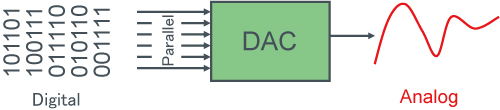
Multi-bit DACs work like this: the PCM stream is split into two channels, left and right, and converted from serial to parallel, for example by shift registers. Data from the right channel is written to the buffer of one register and data from the left channel is written to the buffer of the other. Data is transmitted simultaneously through parallel ports with a certain sample rate (most often 44.1 kHz), as in the picture below, only the parallel outputs are not eight, but sixteen, because the bit width it is 16 bit. Depending on the position in the frame, the high and low bits will encounter different resistances along the path of the electric current, since the number of resistors connected in series will be different. The older the bit, the greater its importance.

Multi-bit, or multi-bit, DACs require very high-quality components and precise resistance adjustment, because any inaccuracies in component ratings add up. This leads to serious deviations from the original waveform and creates a multi-digit error in quantization.

There is no PCM manipulation in multi-bit DACs from the eighties. The multibits are connected directly to the I2S bus and reproduce PCM as is: the data from the right channel (16 bits) arrived, they waited for the data from the second channel (16 bits), they sent both channels to the resistive matrix, and so on with a 44.1 kHz frequency.

In the eighties, the frequency and the bit depth were determined by the CDDA format, which became almost a reference implementation of Kotelnikov’s theorem. With some reservations, this is how the later MP3 can be characterized. Only from the DVD Audio format has the approach to digitizing and sound reproduction been revised.

This is how the first simpler DACs worked, then they began to use converters with a more complex device. Circuitry was modernized, component quality was improved, and multi-bit DAC oversampling technology was also used. Oversampling is the oversampling of a digital stream with upsampling and quantization bit depth to reduce quantization noise.

To explain why oversampling is used, it is necessary to talk about the application of Kotelnikov’s theorem in practice. Not everything here is as optimistic as it seems in the world of mathematics; it is not about anything “precisely”, as it is written in the theorem.

Kotelnikov’s theorem
“Any function F (t), consisting of frequencies from 0 to 1, can be transmitted continuously with any precision using numbers that occur in 1 / (2f 1) seconds”

Consequences of Kotelnikov’s theorem:

Any analog signal can be reconstructed with any precision from its discrete samples taken with a frequency f> 2fc, where fc is the maximum frequency that is limited by the spectrum of the real signal;
If the maximum frequency in the signal is equal to or greater than half the sampling frequency (aliasing), then there is no way to recover the signal from discrete to analog without distortion.
If you are interested in the details, you can consult the main source – the work “On the bandwidth of” ether “and cable in telecommunications” by V. A. Kotelnikov (PDF).

Difficulties with Kotelnikov’s theorem
Kotelnikov’s theorem is often taken too literally and elevated to the absolute. How many articles by staunch skeptics I have read about the wonderful MP3 and CDDA formats and the crazy audiophiles who sell their unnecessary DVD-Audio and DSD to everyone! Of course, your main argument is Kotelnikov’s theorem.

To begin with, the Nyquist frequency, in practice, is not sufficient to transmit an accurate waveform. Due to imperfect conditions, noises and distortions inevitably appear: quantization noise when recording an audio signal, rounding noise during processing and playback, and more.

How does encoding work in digital audio? Part 5

How does encoding work in digital audio? Part 5

encoding digital audio

DSD offers significant advantages over PCM:

encoding digital audio

more precisely draw a wave;
increased immunity to noise;
an easier way to change and transmit a digital stream;
In theory, it is possible to reduce cost by simplifying DAC circuits, but due to backward compatibility, manufacturers are unlikely to do so.
Originally, SACDs used the DSD x64 format with a sample rate of 2822.4 kHz. The 44.1 kHz audio CD sample rate was taken as the basis, increased 64 times, hence the name x64. The following DSDs are currently in use:

x64 = 2822.4 kHz;
x128 = 5644.8 kHz;
x256 = 11,289.6 kHz;
x512 = 22,579.2 kHz;
declared DSD x1024.

DXD
There is a certain intermediate format between PCM and DSD called DXD – Digital eXtreme Definition. This is, in fact, high definition PCM: 352.8 kHz or 384 kHz with 24 or 32 bit quantization. It is used in studies for the processing and subsequent mixing of materials.

But this approach is flawed: firstly, it does not allow to use all the advantages of DSD, and secondly, the file size is larger than in DSD. At the moment, flagship DACs on the I2S input accept a PCM data stream with a sample rate of up to 768 kHz and a bit depth of up to 32 bits. It’s scary to even consider how much hard drive space an album will take up at this resolution.

DSD has practically separated from SACD. Now, the DSD format can often be found packaged in files with the DSF and DFF extensions. Many turntables have been released with the ability to record in DSF and DFF, lovers of good sound are increasingly digitizing vinyl records in the DSD format. But in recording studios, nobody wants to invest in unpopular formats, so they continue to rivet the sound with a minimum wage: 44.1 × 16.

DSD switching and data transmission
To transfer a digital transmission to DSD, a three-pin connection scheme is used:

DSD Clock Pin (DCLK) – sync;
Data input pin DSD Lch (DSDL) – left channel data;
Data input pin DSD Rch (DSDR): Right channel data.

Unlike I2S, DSD data transmission is extremely simplified. DCLK sets the clock rate of the bit sync, and the left and right channel data is transmitted sequentially through the DSDL and DSDR pins, respectively. Here there are no adjustments, recording and playback in DSD is done little by little. This approach provides the closest approximation to the analog signal, and due to the high frequency, the quantization noise is reduced and the reproduction precision is increased by an order of magnitude.

PDO
DoP is often used to carry DSD data streams, so it’s worth mentioning. DoP is an open standard for transferring DSD data over PCM frames (DSD over PCM). The standard was created to transmit a stream through controllers and devices that do not support direct DSD streaming (not native DSD).

The principle of operation is as follows: in a 24-bit PCM frame, the upper 8 bits are padded with ones; this means that DSD data is currently being transmitted. The remaining 16 bits are sequentially filled with DSD data bits.

For x64 DSD transmission with a single bit rate of 2822.4 kHz, a PCM sample rate of 176.4 kHz (176.4 x 16 = 2822.4 kHz) is required. For DSD x128 transmission at 5644.8 kHz, a PCM sampling rate of 352.8 kHz is already required.

How does encoding work in digital audio? Part 4

How does encoding work in digital audio? Part 4

encoding digital audio

When playing PCM 44.1×16, the most significant bits are simply ignored as they are filled with zeros, or, in the case of older multi-bit DACs, they can go to the next frame. The length of the “word” (WS) may also depend on the player through which the music is played, as well as the driver for the playback device.

encoding digital audio

An alternative to PCM and I2S would be to record the audio signal in DSD. This format was developed in parallel with PCM, although Kotelnikov’s theorem had some influence here. To improve sound quality compared to CDDA, the emphasis was not on increasing the quantization bit, as in the DVD Audio format, but on increasing the sample rate.

DSD
DSD stands for Direct Stream Digital. It originates from Sony and Philips labs, however, just like the other formats discussed in this article.

SACD
DSD first saw the light of day on Super Audio CDs in 2002.

At the time, SACD looked like a masterpiece of engineering, applying a completely new way of recording and playback, very close to analog devices. The implementation was simple and elegant.

The media was even equipped with copy protection, although without it, no pirate was afraid. Under the Sony and Philips brands, they began to produce “closed” devices exclusively for playback, with no possibility of copying discs. Manufacturers sold recording equipment to studios, but kept control over the SACD launch.

Who knows, perhaps the SACD format could gain comparable popularity to Audio CD, if it weren’t for the cost of the playback devices. By unreasonably selling out player prices, Sony and Philips’ own leaders stymied the popularity of their format. And the next mistake put an end to the sale of specialized devices. To promote the Sony PlayStation game console, Sony engineers have added the ability to listen to SACD on it. Hackers immediately hacked the set-top box and began to copy SACD discs into ISO images, which can be burned to a regular DVD disc and played on any competing player; others simply ripped out tracks to play on a computer.

Record labels are good too: contrary to what music lovers expected, they did not take full advantage of the new high-definition format. The studios did not record music from the master tape in DSD, instead they took a digital recording in PCM, remixed and processed everything in a row: limiters, compressors, noise-shaping dithering, and various digital filters. The result was a sound so sterile and dry that even CD Audio could have sounded much better. Thus, listeners’ trust in the SACD was undermined, and at the same time in the new formats in general.

INFO
Unfortunately with vinyl records this vicious practice continues to this day: studios print vinyl from a digital recording, even if they have the recording on the master tape. So on modern vinyl it can easily be 44.1 x 16.

DSD
What is DSD? This is a one-bit stream with a very high sample rate compared to PCM. Also, DSD uses a different type of modulation, PDM (Pulse Density Modulation) – pulse density modulation. Sound recording in this format is done by a one-bit analog-to-digital converter, now these ADCs based on sigma-delta modulation are used everywhere. The recording process looks like this: while the amplitude of the wave increases, the output of the ADC is a logical unit, when the amplitude falls, the output is a logical zero, there can be no average value. It is compared with the previous value of the wave amplitude.

How does encoding work in digital audio? Part 3

How does encoding work in digital audio? Part 3

encoding digital audio

The structure of the digital audio path.

encoding digital audio

When playing music, something like the following happens: the player, using a codec created in the form of a device or program, decompresses the file into a specific format (FLAC, MP3 and others) or reads data from a CD, DVD-Audio or disc SACD, receiving a standard PCM data stream … This sequence is then sent via USB, LAN, S / PDIF, PCI, etc. to the I2S converter. In turn, the converter converts the received data into so-called I2S data interface frames (not to be confused with I2C!).

I2S
I2S is a digital audio transmission serial bus. Now I2S is a standard for connecting a signal source (computer, turntable) to a digital-to-analog converter. It is through it that the vast majority of the DAC connects directly or indirectly. There are other digital audio transmission standards, but they are much less common.

I2S output (input) on PCB
Other articles in this issue:
Xakep # 256. Fight Linux
Problem content
Subscription to “Hacker”
The I2S bus can consist of three, four, or even five pins:

continuous serial clock (SCK) – bit sync clock (can be called BCK or BCLK);
word selection (WS) – frame sync clock (may be called LRCK or FSYNC);
serial data (SD): the signal of the transmitted data (can be called DATA, SDOUT or SDATA). As a general rule, data is transmitted from a transmitter to a receiver, but there are devices that can act as a receiver and transmitter at the same time. In this case, another contact may be present;
Serial data in (SDIN): On this pin, data moves in the receive direction, not transmit.
SD or SDOUT is used to connect a D / A converter and SDIN is used to connect an A / D converter to the I2S bus.

In most cases, there is another pin, the master clock (MCLK or MCK), which is used to synchronize the transmitter and receiver from the same clock to reduce the transmission error rate. For external synchronization of MCLK, two clock generators are used: with a frequency of 22 579 kHz and 24 576 kHz. The first, 22,579 kHz, is for frequencies that are multiples of 44.1 kHz (88.2, 176.4, 352.8 kHz), and the second, 24,576 kHz, is for frequencies that are multiples of 48 kHz (96, 192, 384 kHz). There may also be generators at 45158.4 kHz and 49152 kHz; You’ve probably already noticed how in the world of digital sound they like to double everything.

Frame or I2S frame
In I2S, three contacts are necessarily used: SCK, WS, SD; all other contacts are optional.

On the SCK channel, synchronization pulses are transmitted, under which the frames are synchronized.

The length of the “word” is transmitted over the WS channel and logical states are also used. If the WS pin is a logical unit, then the right channel data is transmitted, if it is zero, the left channel data.

The data bits are transmitted via SD: the amplitude values ​​of the audio signal during quantization, the same 16, 24 or 32 bits. No checksums or service channels are provided on the I2S bus. If the data is lost in transit, there is no way to get it back.

Expensive DACs often have external connectors to connect to I2S. The use of such connectors and cables can have a negative effect on the sound, even the appearance of “artifacts” and stuttering, everything will depend on the quality and length of the cable. Still, I2S is a plug-and-play connector, and the length of the wires from the transmitter to the receiver should tend to zero.

Let’s take a look at how the PCM data stream is transmitted over the I2S bus. For example, when transmitting PCM 44.1 kHz at 16 bits, the length of the word on the SD channel will be these sixteen bits and the length of the frame will be 32 bits (right + left). But most of the time, the transmitters use a 24-bit word length.

How does encoding work in digital audio? Part 2

How does encoding work in digital audio? Part 2

digital audio

The 44.1 kHz sampling rate was calculated from Kotelnikov’s theorem. It is believed that the hearing of the average person cannot pick up sound beyond 19-22 kHz. The frequency was probably 22 kHz and was chosen as the upper limit.

digital audio

22,000 × 2 = 44,000 + 100 = 44,100 Hertz

Where does the 100 Hertz come from? There is a version that this is a small margin in case of errors or oversampling. In fact, Sony chose this frequency for its compatibility with the PAL transmission standard.

The bit depth of the CDDA format is 16 bits, or 65,536 samples, which equates to a dynamic range of approximately 96 dB. Such a large number of samples were not chosen by chance. Firstly, due to the strong influence of quantization noise, and secondly, to provide a formal dynamic range superior to that of the main competitors at the time: cassette records and vinyl records. I’ll cover this in more detail in the section on digital to analog converters.

Development of PCM continued on the principle of multiplying by two. Other sample rates appeared: first, the 48 kHz sample rate was added, and then the frequencies based on it were 96, 192, and 384 kHz. The 44.1 kHz frequency was also doubled to 88.2, 176.4 and 352.8 kHz. Bit depth increased from 16 to 24 and then to 32 bits.

The next after CDDA in 1987 appeared the DAT format – Digital Audio Tape. The sample rate was 48 kHz, the quantization bit did not change. And although the format failed, the 48 kHz sample rate has taken hold in recording studios, as they say, due to the convenience of digital processing.

In 1999, the DVD-Audio format was released, which made it possible to record on a disc six stereo tracks with a sampling frequency of 96 kHz and a 24-bit bit depth, or two stereo tracks with a frequency of 192 kHz, 24 bits.

That same year, the SACD – Super Audio CD format was introduced, but the discs began to be produced only three years later. I’ll tell you more about this format in the DSD section.

These are the main formats that are considered the standard for digital audio recordings on media. Now let’s see how the data is transmitted on a digital audio path.

How does encoding work in digital audio?

How does encoding work in digital audio?

encoding digital audio

Have you ever wondered how sound is reproduced on digital devices? How is a sound signal formed from a combination of ones and zeros?

encoding digital audio

I’m sure I was thinking, since I started reading! But often, even professionals have only a general idea of ​​the modern sound route. In this article, you will learn how the different formats appeared, what a digital-to-analog converter is, what types of DACs exist, and what determines the quality of sound reproduction.

PCM
As you know, in digital audio, almost any format, with rare exceptions, is recorded using a pulse code stream or a PCM stream – pulse code modulation. FLAC, MP3, WAV, Audio CD, DVD-Audio and other formats are just ways to pack, “preserve” the PCM stream.

How it all began
The theoretical foundations of digital sound transmission were developed at the dawn of the 20th century, when scientists tried to transmit an audio signal over a long distance, but not by telephone, but in a rather strange way for that time.

By dividing the sound wave into small parts, it could be sent to the receiver in some kind of mathematical representation. The recipient, in turn, could restore the original waveform and listen to the recording. In addition, scientists were faced with the task of increasing the bandwidth of the “ether”.

In 1933, the theorem of V.A. Kotelnikov. In Western sources, it is called the Nyquist-Shannon theorem. Yes, Harry Nyquist was the first to raise this issue: in 1927 he calculated the minimum sampling frequency for transmitting a waveform, which later received his name “Nyquist frequency”, but Kotelnikov’s theorem was published 16 years earlier .

The essence of the theorem is simple: a continuous signal can be represented in the form of an interpolation series consisting of discrete reports, from which the signal can be reconstructed. In order to roughly restore the original state of the signal, the sample rate must be at least twice the upper cutoff frequency of this signal.

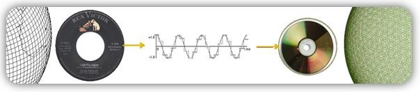
For many years, the theorem was not in demand, until the advent of the digital age. It was then that it found a use. In particular, the theorem was useful in the development of the CDDA (Compact Disc Digital Audio) format, in common people it is called Audio CD or Red Book. The format was released by engineers at Philips and Sony in 1980 and has become the standard for audio CDs.

Format characteristics:

sampling frequency – 44.1 kHz;
quantization capacity – 16 bits.

Where did 44100 come from

Where did 44100 come from

44100

The standard sample rate for CD-audio is 44100 Hertz. Where and why were these 44100s originally chosen for CD audio production?

44100

Starting from the condition (see Nyquist-Shannon-Kotelnikov) of reproduction of the upper limit of the spectrum at 20 kHz, the sampling frequency should have been chosen above 40 kHz. But at the time of the creation of these standards and the development of CD-DA technology (the second half of the 70s of the last century), there was no generally accepted medium in which to record, edit and store digital sound. And for this, it was decided to use standard VCRs, which in those days worked in U-matic format. The digital signal was encoded by a special encoder into a black and white video pseudo-signal and recorded on a video cassette. The structure of the digital signal had to be linked to the frequency and structure of the fields of the television signal used for recording.

This decision was complicated by the fact that different video recording standards are used in Europe and the US: 525 lines at 60 Hz and 625 lines at 50 Hz, while not all lines can be used to record information. The selected frequency should fit the structure of both video signals. 44100 Hz meet this requirement.

In a 60 Hz NTSC video signal, 35 lines are not used for recording, leaving 490 active lines per frame, or 245 in the field for digital audio recording. When writing three samples to a string, the sample rate will be:

60 × 245 × 3 = 44100.

In a 50Hz PAL signal, 37 lines are not used, leaving 588 active lines per frame, or 249 per field, so the frequency will be:

50 × 249 × 3 = 44100.

Although digital sound at that time had nothing to do with the video signal, video equipment was used in the production of the CD, which determined the choice of sampling frequency.

Analog to digital signal conversion Part 3

Analog to digital signal conversion Part 3

Analog to digital

Keywords can be streamed in parallel or serial.

Analog to digital

For parallel transmission, n communication lines must be used (n = 4). The codeword symbols are transmitted simultaneously over the lines within the sampling interval. For serial transmission, the sampling interval must be divided into n subintervals: cycles. In this case, the characters of the word are transmitted sequentially along a line and a clock cycle is assigned for the transmission of one character of the word. Each character of the word is transmitted by one or more discrete signals: pulses. Therefore, converting an analog signal into a sequence of code words is often called pulse code modulation. The way words are represented by certain signals is determined by the format of the code. You can, for example, set the signal level high within the clock cycle if a binary character 1 is transmitted in this clock cycle, and low – if a binary character 0 is transmitted (this representation method, shown in the Fig. 6, it is called BVN format – No return to zero).

In the example of Fig. 6 it uses 4-bit binary words (this allows 16 levels of quantization). In a parallel digital stream, 1 bit of a 4-bit word is transmitted on each line within the sampling interval. In a serial stream, the sampling interval is divided into 4 clocks, in which the bits of a 4-bit word are transmitted (starting with the most significant). 6 uses 4-bit binary words (this allows 16 levels of quantization). In a parallel digital stream, 1 bit of a 4-bit word is transmitted on each line within the sampling interval. In a serial stream, the sampling interval is divided into 4 clocks, in which the bits of a 4-bit word are transmitted (starting with the most significant). 6 uses 4-bit binary words (this allows 16 levels of quantization). In a parallel digital stream, 1 bit of a 4-bit word is transmitted on each line within the sampling interval. In a serial stream, the sampling interval is divided into 4 clocks, in which the bits of a 4-bit word are transmitted (starting with the most significant).

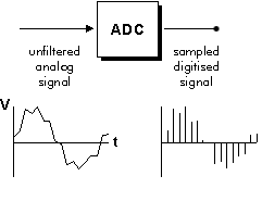
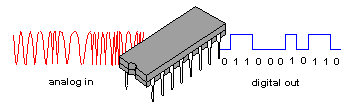
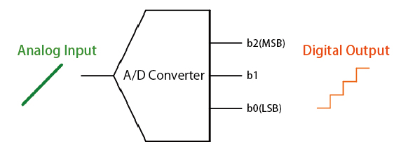
Operations related to converting an analog signal to digital form (sampling, quantizing, and encoding) are performed by one device: an analog-to-digital converter (ADC). Today, an ADC can simply be an integrated circuit. Reverse procedure, ie restoring an analog signal from a sequence of code words is performed in a digital-to-analog converter (DAC). Now there are technical possibilities for implementing all image and sound signal processing, including recording and transmission, in digital form. However, analog devices are still used as signal sensors (for example, a microphone, a TV transmission tube, or a charge-coupled device) and sound and image reproduction devices (for example, a speaker, a kinescope ).

Digital signals can be described using typical parameters of analog technology, such as bandwidth. But its applicability in digital technology is limited. An important indicator characterizing digital flow is the data transfer rate. If the length of the word is n and the sampling rate is FD, then the data rate, expressed in the number of binary symbols per unit time (bit / s), is calculated as the product of the length of the word by the sampling frequency: C = nFD.

Analog to digital signal conversion Part 2

Analog to digital signal conversion Part 2

Analog to digital

If you need no distortion of the TV signal during the sampling process with a cutoff frequency, for example 6 MHz, then the sampling frequency must be at least 12 MHz.

Image result for Analog to digital

However, the closer the sample rate is to twice the cutoff frequency of the signal, the more difficult it is to create a low-pass filter, which is used in the reconstruction and also in the pre-filtering of the original analog signal. This is due to the fact that as the sampling frequency approaches the doubling cutoff frequency of the sampled signal, increasingly stringent requirements are imposed on the shape of the frequency characteristics of the reconstruction filters: it must correspond more and more precisely to a rectangle. characteristic. It should be noted that a rectangular filter cannot be physically implemented. Such a filter, as theory shows, must introduce an infinitely large delay into the transmitted signal. Therefore, in practice, there is always a certain interval between the doubled cutoff frequency of the original signal and the sampling frequency.

Quantification
– represents the replacement of the count value of the signal with the closest value of a set of fixed values ​​- quantization levels. In other words, quantization is the rounding of the count value. Quantization levels divide the entire range of possible changes in signal values ​​into a finite number of intervals: quantization steps. The location of the quantization levels is determined by the quantization scale. Uniform and non-uniform scales are used. In Fig. 3 shows the original analog signal and its quantized version obtained by means of a uniform quantization scale, as well as the corresponding image signals.

Signal distortions that occur during the quantization process are called quantization noise. In instrumental noise estimation, the difference between the original signal and its quantized copy is calculated and, for example, the root mean square value of this difference is taken as objective noise indicators. The timing diagram and the image of the quantization noise are also shown in Fig. 3 (the image of the quantization noise is shown on a gray background). Unlike jitter noise, quantization noise is correlated with the signal, so quantization noise cannot be removed by post-filtering. The quantization noise decreases as the number of quantization levels increases.

With a relatively large number of levels, the quantization noise is similar to the usual jitter noise. The noise oscillation was reduced, so it was necessary to increase this oscillation 128 times when obtaining an image of quantization noise to make the noise noticeable. A few years ago, it seemed sufficient to use 256 levels to quantify a television video signal. It is now considered the norm to quantify a video signal at 1024 levels. The number of quantization levels in the formation of a digital audio signal is much greater – from tens of thousands to millions.

Digital encoding
A quantized signal, unlike the original analog signal, can only take on a finite number of values. This allows a number equal to the ordinal number of the quantization level to be represented within each sampling interval. In turn, this number can be expressed by a combination of some signs or symbols. The set of characters (symbols) and the system of rules by which data is represented as a set of characters is called a code. The final sequence of code symbols is called a code word. The quantized signal can be converted into a sequence of code words. This operation is called encoding. Each codeword is transmitted within a sampling interval. Binary code is widely used to encode audio and video signals. If the quantized signal can take N values, then the number of binary symbols in each codeword is n> = log2N. A bit, or character in a word represented in binary code, is called a bit. Generally, the number of quantization levels is equal to an integer power of 2, that is, N = 2n.