Tag: a/d and d/a converters in embedded systems

Free Download Mp4Gain

Noise – Part 4

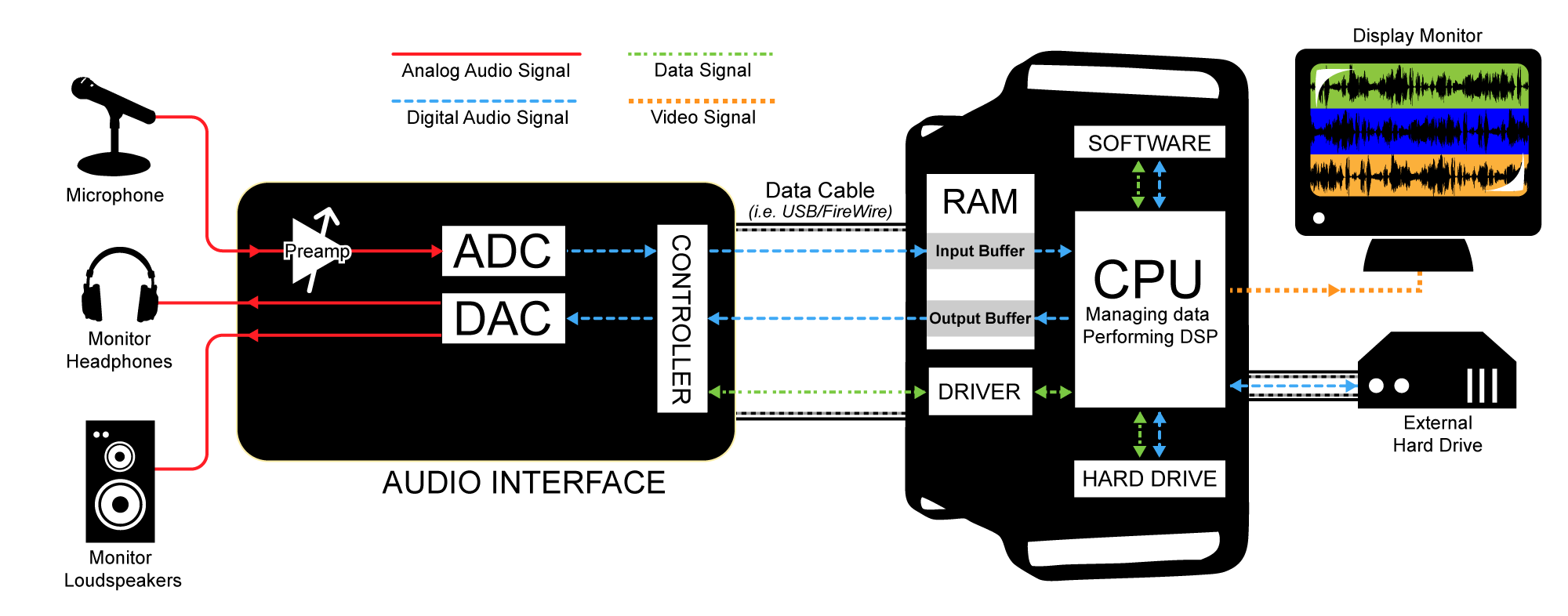
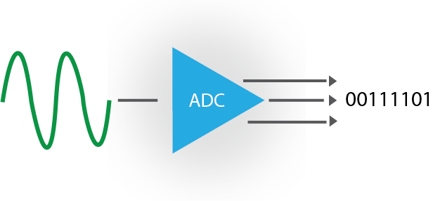
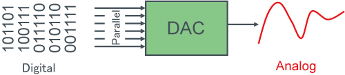
To summarize and simplify, something like the following happens. A PCM data stream is fed to the DAC input through the I2S connector, oversampling is added, dithering, and then the stream is sent to a noise shaping decoder. At the end, a one-bit stream is formed, it passes through an analog low-pass filter, where the final audio signal that we hear is already obtained.

A multi-bit DAC is more complex: in addition to the above, it also uses DEM technology.

WWW
If you want to understand the details, please read the materials in the links, there is information not only about sigma-delta-DAC, but also about sigma-delta-ADC.

Article on delta-sigma modulation on microsin.net
Notes from E. I. Vologdin’s lecture on sigma-delta modulation
Modern digital-to-analog converters are complex devices. But the use of these technologies is necessary to artificially expand the dynamic range, and they are generally used to overcome the limitations of CDDA and MP3 formats. If the recordings were originally published in high resolution PCM (192 × 24), or better in DSD format, then there would not be as many technologies and complex digital transformations. In the case of DSD, interference with the quantized signal is not necessary at all, at least during playback.

Conclution
The development of recording and playback in the digital age has been challenging and arduous. With the invention of the compact disc, analog audio practically ceased to exist in just a couple of decades. Good or bad: everyone decides for themselves, but I would like the possibility to choose to remain. If it is not between digital and analog, at least how and with what quality to listen to your favorite music. Unfortunately, now there is hardly any other option. Few people are releasing high definition music these days, aside from crawler enthusiasts. The only fault for this is the recording studios, who decided to limit themselves to a single format: CDDA.

All that’s left is to sympathize with the musicians! How much effort and time they put into creating music, but their work isn’t even preserved in decent quality. The solution would be to record on the master tape or at least on DSD. But the recording studios will not waste extra effort, because they are satisfied with the current situation (PDM).

Free Download Mp4Gain


Mp4Gain Main Window


Mp4Gain Features


Free Download Mp4Gain

Noise – Part 3

In addition to those considered, other technologies are used, as well as their combinations and variations.

Manufacturers especially love experimenting with digital filters and modulators, inventing more and more digital filters that affect the signal for both better and worse. Modern DAC digital signal processing algorithms are often complex and include all of the above, as well as manufacturers’ own developments. Of course, manufacturers do not publish algorithms for filters and modulators; at best, they provide a rough block diagram. Therefore, it remains only to assume what actually happens with the audio signal inside one or another digital-to-analog converter.

Sigma delta converters
Sigma-delta digital-to-analog converters have evolved apart from multi-bit DACs. The base was taken, as its name indicates, sigma-delta modulation, in the literature it is usually denoted by the abbreviation SDM. In sigma-delta modulation, the absolute value of the signal amplitude is not transmitted per unit time, as in multi-bit DACs, but the signal changes from the previous value. So if the amplitude increases, 1 is transmitted, and if it falls – 0. A similar principle was already described in the section on DSD.

Early sigma-delta DACs were completely 1-bit, but due to the high sample rate, they provided a dynamic range of approximately 129 dB. The sampling frequency is 44.1 kHz. The chosen frequency probably saved hardware resources due to simplification of calculations during interpolation.

At the beginning, a frequency of 2.8 MHz was used, this is 44.1 kHz, increased 64 times. Now the frequency can be different, it is determined by the internal architecture of the DAC itself. It is generally based on frequency grids in multiples of 44.1 kHz and 48 kHz, with a multiplier of 64, 128, 256, 512, 1024.

Over time, delta-sigma DACs have almost completely supplanted multibit, simply for economic reasons. First, its component quality and precision requirements are much lower than multi-bit DACs, and consequently the cost price is lower. Second, in the 1980s and 1990s, the cost of implementing interpolation and noise shaping for a one-bit modulator was significantly less than for 16-bit. Now, with the development of technology, this is not that critical, and many sigma-delta DACs, like multibits, have multiple levels of output. But due to the multiple increase in frequency, the requirements for the components are not still very high, so the first advantage continues to this day.

Modern sigma-delta DACs are complex and include almost all of the technologies listed in the previous chapter. I will give an example of the internal structure of one of the simple sigma-delta-DACs from the Vologdin lectures.

Input 16-bit digital samples with a sampling frequency of 44.1 kHz are fed into the digital oversampling filter. The scheme uses a non-recursive quadruple oversampling FIR (finite impulse response) interpolation filter with a linear phase response. In the first modulation stage, as a result of requantization, the number of bits in the samples is reduced from 16 to 14 and first-order SDM is used. Then a further resampling is performed using two steps (Kos = 32 and 2). A noise signal is introduced on the path between these stages, performing the “Dithering” operation with a noise level equal to minus 20 dB. It reduces the non-linearity of the transfer function due to quantization errors. The overall oversampling factor is 256 and the sampling frequency increases to 11.29 MHz. In the second modulation stage, second-order SDM is used and a one-bit digital stream is formed. The DAC output is connected to a digital time pulse modulator, which converts the digital data into a density modulated pulse sequence (PDM).

Noise – Part 3

Recording audio

To record and mix the audio signal, they started using decimation, this is the reverse process, oversampling with downsampling and quantization bit depth. The signal is recorded at a high sample rate and quantization bit depth, for example 176.4 or 192 kHz with a 24 bit bit depth, and removing some of the samples using a digital filter is “compressed” to the CDDA standard – 44.1 kHz, 16 bits. This approach can slightly reduce quantization noise.

Below is an illustration of the algorithm for decimating a discrete signal with a factor of 2. Red dots indicate samples, solid lines – a continuous signal, representing these samples. Above is the original signal. In the middle, the same signal after filtering on a digital low pass filter. Below is the decimated signal.

Dithering
Dithering (dithering) – A method of mixing pseudo-random noise when digitizing or playing a sound signal. This technology has two purposes:

linearization of the quantizer / requantizer transfer function;
decorrelation of quantization errors.
Quantization noise has a correlation, that is, a relationship with the main signal. This creates parasitic harmonics that follow the waveform. They affect perception creating a “diffuse” sound. Correlation can be removed by adding specially patterned noise to the main signal, thus converting the correlated quantization noise to ordinary white noise. This increases the overall noise level a bit, but is good for perception.

Dithering in the image processing example: before and after
Dithering in the image processing example: before and after
Noise modeling
Noise Shaping (NS) technology can significantly reduce noise introduced during quantization, re-entrapment, and dithering.

Noise modeling works like this: the quantized signal at the input is compared to the signal at the output of the requantizer, a difference (error) is formed, which is subtracted from the main signal. This compensates for distortions introduced by the requantizer and during the dithering process. A so-called feedback is formed, which seeks to compensate for the error in the input and output of the requanter. This technology works like negative feedback in an op amp, except that all conversions are done digitally.

Here’s a diagram of a first-order requantizer, but as a rule, requanters are used up to order 9-12.
Here’s a diagram of a first-order requantizer, but as a rule, requanters are used up to order 9-12.
This technology has its drawbacks. Using NS introduces a large amount of noise in the high frequency region, making it necessary to apply a low pass filter, with a cutoff frequency close to the upper cutoff frequency. In practice, together with NS, dithering is also always used, the result of their joint work is much better by ear.

Dynamic item matching
Dynamic Element Matching (DEM) is a technology that generates various signal levels at the DAC output. It looks like a cross between a single bit and multi-bit DAC. DEM is used to reduce deterministic errors when using sigma-delta modulation (SDM). These errors, like quantization noise, are highly correlated with the signal at the one-bit modulator output and therefore significantly affect the perception of the audio signal.

This technology also reduces the requirements for the analog filter, because the waveform is close to the reproduced waveform even before filtering. DEM is implemented with several pins connected to a common bus, which form the output signal of the DAC.

Noise – Part 2

Also, poor sound engineers love to shake and level everything using limiters and compressors, the principle of which is based on reducing the dynamic range.

Almost all samples go through all this torture. Even when using a simple EQ, the signal passes through a digital filter, which introduces rounding noise by at least half a quantization step. During final mixing, all samples are collected in a sequence, respectively, the noise from each being added to the noise from another resampling. But that’s not all: during playback, the DAC adds its own noise and rounding noise. Can you imagine what really remains of the useful signal?

Noise control techniques
To remedy this unfortunate situation, special noise reduction technologies have been developed. Let’s see the most basic.

Oversampling
Oversampling technology has been used since the days of multi-bit DACs to compensate for losses caused by noise. The principle of oversampling is that intermediate samples are added to existing discrete samples, repeating the approximate waveform. Intermediate samples are calculated by mathematical interpolation or filled with zero values ​​and transmitted to a digital filter. Generally, both approaches are called interpolation and the digital filter is called interpolation. The simplest interpolation method is linear interpolation, and the simplest digital filter can be a low-pass filter.

Below is an illustration of an interpolation algorithm for a discrete signal with a factor of 2. Red dots indicate the original signal samples, solid lines – a continuous signal, representing these samples. Above is the original signal. In the middle is the same signal with inserted zero counts (green dots). Bottom: interpolated signal (blue dots: interpolated sample values).

At first they started using only oversampling with an increase in frequency, for example from 44.1 to 176.4 kHz. Subsequently, oversampling was used with an increase in the sampling frequency and an increase in the quantization bit depth; This process is called recantization.

Although oversampling introduces rounding noise, it also reduces overall noise density by expanding the dynamic range of the signal, and post-processing of the signal will have less impact. Each doubling of the sample rate expands the dynamic range by approximately one quantization step (6 dB) minus the rounding noise.

Just to be able to use oversampling, they began to produce multi-bit DAC chips that supported up to 192×24 digital stream on input. DSP (digital signal processor) -based hardware upsamplers also appeared.

Of course, the use of oversampling technology improved the characteristics of the audio signal, but the situation did not change drastically: the noise level remained high. Therefore, other technologies began to be applied.

Noises

There are many types of noise that can affect recording. These are the main ones: quantization noise, rounding noise, aperture jitter, harmonic distortion, analog noise.

You can familiarize yourself with the descriptions of the four types of noise and the formulas to understand approximately how much distortion each type introduces into a digitized signal.

Do not take the term “noise” as a manifestation of the well-known “white noise”. Different types of noise are perceived differently, in this context the term “noise” should be understood rather as the loss of a part of the useful signal.

It is still possible to roughly calculate one type of noise separately, but the general noise level during digitizing is hardly. This is a very complex mathematical model with many assumptions. Let’s try to go from the opposite and analyze the dynamic range of the signal recorded in the ADC (analog-digital converter) and compare it with what is theoretically possible.

The noise level is generally calculated in relation to the quantization step (one bit) or the dynamic range of the audio signal. The dynamic range is measured in decibels, it can be calculated by the formula: DR = 20lg (2 N), where N is the quantization bit. It turns out that for 16 bits the possible dynamic range is about 96 dB and for 24 bits about 144 dB.

I will take the results of testing the ADC “Lynx Studio Hilo TB”, this is a studio ADC / DAC of the highest price category. It showed the following results.

WORKING HOURS 24 BITS, 44 KHZ
Dynamic range, dB (A) 119.3 Fine
And here are the results without amplification.

WORKING HOURS 24 BITS, 44 KHZ
Dynamic range, dB (A) 112.6 Fine
Looking ahead, I will say that the tested ADC uses Dithering, Noise Shaping, and Decimation technologies, allowing for expanded dynamic range and reduced noise level. I will tell you more about these technologies in the next paragraph.

Now let’s estimate: 24 bits equals 144 dB; this is the possible dynamic range. We subtract the actual dynamic range of 119 dB from 144 dB, the noise loss will be 25 dB at best and 32 dB at worst. Unfortunately, it was not tested at 16-bit, but in terms of the ratio, the results should be even worse, since reducing the bit depth inevitably leads to increased noise. It turns out that about 1/5 of the signal is simply lost due to noise.

The picture is far from rosy. And if you dig deeper and consider how the sound is mixed in the recording studio, it becomes awkward. As a general rule, finished work is mixed from samples where the indicated noises are already present, as the samples are recorded on a similar ADC. Effects are then added that at least lead to resampling and associated rounding errors.

D / A converters

Let’s move on to DAC: digital to analog converters. This complex subject is always covered with a veil of secrecy and peppered with audiophile mysticism.

Additionally, there is a lot of speculation from opposing camps around digital-to-analog converters: marketers, audiophiles, and skeptics. Let’s find out what the problem is.

Multibit DAC
In the beginning when the audio CD format first appeared, PCM was converted to an analog signal using multi-bit DACs. They were built on the basis of a resistive matrix with constant impedance, the so-called R-2R matrix.

Simplified multi-bit DAC circuit
Simplified multi-bit DAC circuit
Multi-bit DACs work like this: the PCM stream is split into two channels, left and right, and converted from serial to parallel, for example by shift registers. Data from the right channel is written to the buffer of one register and data from the left channel is written to the buffer of the other. Data is transmitted simultaneously through parallel ports with a certain sample rate (most often 44.1 kHz), as in the picture below, only the parallel outputs are not eight, but sixteen, because the bit width it is 16 bit. Depending on the position in the frame, the high and low bits will encounter different resistances along the path of the electric current, since the number of resistors connected in series will be different. The older the bit, the greater its importance.

Multi-bit, or multi-bit, DACs require very high-quality components and precise resistance adjustment, because any inaccuracies in component ratings add up. This leads to serious deviations from the original waveform and creates a multi-digit error in quantization.

There is no PCM manipulation in multi-bit DACs from the eighties. The multibits are connected directly to the I2S bus and reproduce PCM as is: the data from the right channel (16 bits) arrived, they waited for the data from the second channel (16 bits), they sent both channels to the resistive matrix, and so on with a 44.1 kHz frequency.

In the eighties, the frequency and the bit depth were determined by the CDDA format, which became almost a reference implementation of Kotelnikov’s theorem. With some reservations, this is how the later MP3 can be characterized. Only from the DVD Audio format has the approach to digitizing and sound reproduction been revised.

This is how the first simpler DACs worked, then they began to use converters with a more complex device. Circuitry was modernized, component quality was improved, and multi-bit DAC oversampling technology was also used. Oversampling is the oversampling of a digital stream with upsampling and quantization bit depth to reduce quantization noise.

To explain why oversampling is used, it is necessary to talk about the application of Kotelnikov’s theorem in practice. Not everything here is as optimistic as it seems in the world of mathematics; it is not about anything “precisely”, as it is written in the theorem.

Kotelnikov’s theorem
“Any function F (t), consisting of frequencies from 0 to 1, can be transmitted continuously with any precision using numbers that occur in 1 / (2f 1) seconds”

Consequences of Kotelnikov’s theorem:

Any analog signal can be reconstructed with any precision from its discrete samples taken with a frequency f> 2fc, where fc is the maximum frequency that is limited by the spectrum of the real signal;
If the maximum frequency in the signal is equal to or greater than half the sampling frequency (aliasing), then there is no way to recover the signal from discrete to analog without distortion.
If you are interested in the details, you can consult the main source – the work “On the bandwidth of” ether “and cable in telecommunications” by V. A. Kotelnikov (PDF).

Difficulties with Kotelnikov’s theorem
Kotelnikov’s theorem is often taken too literally and elevated to the absolute. How many articles by staunch skeptics I have read about the wonderful MP3 and CDDA formats and the crazy audiophiles who sell their unnecessary DVD-Audio and DSD to everyone! Of course, your main argument is Kotelnikov’s theorem.

To begin with, the Nyquist frequency, in practice, is not sufficient to transmit an accurate waveform. Due to imperfect conditions, noises and distortions inevitably appear: quantization noise when recording an audio signal, rounding noise during processing and playback, and more.