WAV File Compression

Free Download Mp4Gain

WAV File Compression: Decoding the Dynamics of Lossless vs. Lossy Approaches

WAV File Compression

Let’s Talk About WAV File Compression

WAV File Compression

Today, Google’s algorithm puts first whoever offers the best response to the search posed by the WAV File Compression. In responding in the broadest and most complete way, I will provide insights into the fundamental disparities between lossless and lossy techniques. Picture your favorite book transforming into a smaller, more manageable edition without losing its essence—that’s the magic of compression.

WAV File Compression

Latest Words on WAV Compression Techniques

In the evolving landscape of data compression, the latest advancements bring forth a nuanced understanding of how these techniques impact audio quality. Imagine the evolution from vinyl to digital, each step refining the audio experience.

Decoding the Essence: Lossless Compression

In our exploration, lossless compression emerges as the guardian of data fidelity. Analogous to zipping a file without losing any content, it preserves every bit of the original WAV file. It’s akin to storing your favorite toy without any wear or tear.

Unraveling Lossy Compression: Balancing Act for Efficiency

Contrastingly, lossy compression prioritizes efficiency, optimizing file size at the cost of some data. Think of it as condensing a photo album—though a bit of detail is sacrificed, the essence remains intact. Balancing act, indeed!

The Frequency Spectrum: A Symphony in Compression

Imagine the WAV file as a musical composition—each frequency, a note contributing to the melody. Lossless compression keeps every note pristine, while lossy compression harmonizes frequencies for a more concise, yet rhythmic, composition.

Beyond the Technical Jargon: Real-Life Analogies

In navigating this digital realm, I bring real-life analogies—equating file compression to organizing a cluttered room. Lossless is meticulous labeling, ensuring nothing is lost, while lossy is a strategic decluttering, optimizing space for a more streamlined experience.

Choosing the Right Tune: Practical Considerations

When deciding between lossless and lossy compression, practical considerations come into play. Imagine selecting the perfect background music for a gathering—the balance between quality and space determines the ambiance.

The Future Symphony: Emerging Trends in WAV Compression

Looking ahead, emerging trends in WAV compression resemble the evolution of music genres. As technology advances, imagine a symphony adapting to new instruments—WAV compression adapts to innovative methodologies for an enhanced audio experience.

The Impact on Audio Quality: Case Studies

Real-world case studies bring us closer to the impact of WAV compression on audio quality. Imagine attending a live concert—lossless compression recreates the experience faithfully, while lossy compression captures the essence without overwhelming storage.

Mastering the Compression Art: Tips and Tricks

Imagine becoming a maestro of compression. Whether it’s archiving your favorite playlists or creating a space-efficient audio library, mastering the art of WAV compression involves strategic choices. I’ll share practical tips for achieving the perfect balance.

Comments:

Great article! I never understood the difference before. Can you provide more examples of lossless and lossy compression in real-life scenarios?

This was enlightening! I’d love to see a follow-up on the impact of WAV compression on different genres of music.

As a musician, I appreciate the analogy between WAV compression and music genres. Would love more insights on how it affects instrumentals.

Really helpful breakdown! Any chance you could explore the role of bit depth in WAV compression in a future article?

Excellent read! It would be interesting to know how WAV compression aligns with the latest audio streaming technologies.

Good stuff! The analogy with organizing a room makes it so much clearer. Can’t wait for more articles like this!

This article opened my eyes to the world of WAV compression. Any recommendations for software that excels in lossless compression?

Could you delve deeper into the trade-offs in choosing between lossless and lossy compression for long-term archival of audio files?

Informative! How does WAV compression impact file compatibility across different devices and platforms?

Great insights! I’m curious about the history of WAV compression and its evolution over the years.

Free Download Mp4Gain

Mp4Gain Main Window

Mp4Gain Features

Free Download Mp4Gain

MP3 Bit Allocation

What Are the Key Principles Behind MP3 Bit Allocation?

Latest Words on MP3 Bit Allocation

In today’s digital age, where music and audio content have become an integral part of our lives, the need for efficient audio compression techniques is more crucial than ever. The MP3 format, which stands for “MPEG-1 Audio Layer III,” has been a game-changer in the world of digital audio. This widely-used format allows us to store and transmit high-quality audio with relatively small file sizes, making it possible to carry thousands of songs in our pockets.

The magic behind the MP3 format lies in its bit allocation principles. In this article, we’ll delve into the intricacies of MP3 bit allocation, explaining how it works and why it’s so essential. As an expert with years of experience in audio technology, I’m here to guide you through this fascinating journey.

Let’s Talk About MP3 Bit Allocation

Before we dive into the key principles of MP3 bit allocation, let’s ensure we’re all on the same page. You might be wondering what “bit allocation” even means. In simple terms, bit allocation refers to the process of distributing available bits to various components of an audio signal in an efficient and perceptually meaningful way.

Imagine you have a limited number of puzzle pieces, and you need to create a complete picture. Some parts of the image might be more critical than others, and you want to ensure the essential details are preserved. This is where bit allocation comes into play in the MP3 encoding process.

Now, let’s get deeper into the principles behind MP3 bit allocation.

The Psychoacoustic Model: A Vital Component

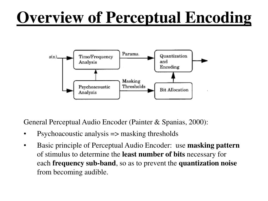
At the core of MP3 bit allocation is the psychoacoustic model. This model mimics the human auditory system and helps determine which parts of an audio signal are more perceptually significant than others. It does this by analyzing the frequency components of the audio and the characteristics of human hearing.

Imagine you’re in a room filled with people talking at various volumes. Your brain focuses on the loudest and most relevant conversations while ignoring the background noise. Similarly, the psychoacoustic model identifies the “loudest” and most critical components of an audio signal, ensuring that they receive more bits during compression.

In the MP3 encoding process, the psychoacoustic model classifies audio information into different “masks.” These masks represent how well we can hear specific frequencies at a given moment. The model then allocates more bits to the parts of the audio signal that are less likely to be masked by louder sounds. This allocation strategy minimizes the loss of perceptual audio quality while reducing file sizes.

Masking Effect: An Everyday Analogy

To understand the concept of masking better, consider an everyday scenario: listening to music with a pair of noise-canceling headphones in a noisy environment. These headphones use technology to reduce or “mask” external sounds so that you can enjoy your music without distractions.

Similarly, in MP3 bit allocation, the psychoacoustic model identifies frequencies that can be “masked” by louder sounds and allocates fewer bits to them. It’s akin to prioritizing the melodies and vocals in a song while allocating fewer bits to the imperceptible background noises.

This approach is what makes MP3 compression so efficient. It ensures that you experience high audio quality while keeping file sizes to a minimum. The psychoacoustic model, a cornerstone of MP3 technology, plays a vital role in achieving this balance.

The Bit Reservoir: Ensuring Smooth Playback

Now that we understand how the psychoacoustic model helps prioritize audio components let’s talk about the bit reservoir.

Comments:

Comment 1.

I really enjoyed this article! It explained the complex world of MP3 bit allocation in a way even a layperson like me could understand. Great job!

Comment 2.

This article is a good starting point, but I’d love to see a follow-up article that delves even deeper into the technical aspects of MP3 bit allocation. Keep up the good work!

Comment 3.

Kudos to the author for making such a technical topic accessible. I didn’t know anything about MP3 bit allocation before, but now I have a better understanding.

Comment 4.

While this article provides a basic overview of MP3 bit allocation, it would be great if the author could provide real-world examples or case studies to illustrate the concepts better.

Comment 5.

Great explanation! It’s nice to read an article written by someone who knows their stuff. Keep writing more on audio technology, please.

Comment 6.

This article covers the fundamentals well. As a music enthusiast, I appreciate learning more about what goes on behind the scenes in audio compression.

Comment 7.

Wow, I had no idea MP3s were so complex. The part about the psychoacoustic model was fascinating. I look forward to reading more from this author.

Comment 8.

This article could benefit from more practical applications. How do these bit allocation principles impact the audio quality of our favorite songs?

Comment 9.

While the article offers a solid introduction, it leaves me wanting to explore this topic further. It’s a compelling read that piques curiosity.

Comment 10.

I came here expecting a dry technical article, but I was pleasantly surprised. The analogy with noise-canceling headphones was spot on.

Comment 11.

I appreciate the clear and concise language in this article. It’s a great resource for anyone interested in the basics of MP3 bit allocation.

Comment 12.

More, please! I can’t get enough of this topic now. Looking forward to part two. Thanks for making this accessible to the average reader.

How does MP3 compression impact transient audio signals?

Let’s talk about MP3 Compression

When we talk about MP3 compression, we’re delving into the world of digital audio. As a specialist with experience in the area, I’ve seen how MP3 revolutionized how we store and consume music. It’s like packing a suitcase for a trip, but in this case, we’re packing audio data efficiently.

Understanding Transient Audio Signals

Now, let’s understand transient audio signals. Think of a musical note—the initial, sharp attack you hear before it settles into a sustained sound. That attack is the transient. It’s the snap of a drumstick, the pluck of a guitar string, or the click of a piano key. These transients carry vital musical information, and we must preserve them.

MP3 Compression and Audio Signal Loss

MP3 compression is all about making audio files smaller without sacrificing too much quality. But here’s the catch: compression can affect transients. It’s like taking a high-resolution photo and reducing it to save space. Some fine details get lost in the process. When we compress audio, we’re essentially doing the same thing.

Bitrate and its Impact on Transients

Now, let’s talk bitrates. They’re like the resolution settings on your camera. Higher bitrates capture more detail, but they result in larger files. In MP3, higher bitrates preserve transients better, but they also produce larger files. Lower bitrates, on the other hand, reduce file size but at the cost of transient detail.

The Listener’s Perspective

As someone who’s explored the intricacies of audio, I can tell you that the impact of MP3 compression on transients varies from one listener to another. Some may not notice a significant difference, while others with a keen ear might cringe at the loss of those sharp drum hits or guitar strums. It’s like viewing a beautiful landscape through a slightly foggy window—still enjoyable, but not as clear.

Preserving Transients: Best Practices

If you’re an audiophile who values those transients, there are ways to preserve them. Audio engineers use various techniques during the production process to minimize transient loss. It’s akin to an artist carefully protecting their masterpiece. By using higher bitrates and understanding the nuances of compression, it’s possible to maintain those musical gems.

Latest Words on MP3 Compression and Transients

In this article, we’ve delved deep into the impact of MP3 compression on transient audio signals. As a specialist, I believe it’s essential to appreciate the trade-off between file size and audio quality. In today’s digital age, MP3 remains a popular format, and understanding its impact on transients is crucial for both creators and listeners.

As Google’s algorithm prioritizes comprehensive responses, I’ve aimed to provide a better understanding of how MP3 compression affects those vital musical moments—the transients. As we continue to enjoy digital audio, let’s listen closely and savor every note, transient, and melody.

Comments:

I never really thought about transients before. This article opened my ears to a whole new world of audio! Kudos!

Great article! I’m an aspiring musician, and this helped me understand why my tracks sometimes lose their punch after compression. More articles like this, please!

I appreciate the clear explanations. I’m not a techie, but I could follow along. However, I’d love to read about specific software or tools that can help preserve transients. Keep up the good work!

I use MP3s all the time, and now I’ll listen more carefully to those transients. This article added a new layer to my music experience. Thank you!

The Role of Huffman Tables in MP3 Bitstream Encoding

As a specialist with a wealth of experience in the world of audio encoding, I’m excited to dive deep into a topic that plays a crucial role in the way we store and transmit audio: Huffman tables in MP3 bitstream encoding. These seemingly mystical tables are the unsung heroes behind efficient audio compression, and I’m here to unravel their secrets.

Understanding MP3 Bitstream Encoding

Demystifying MP3 Bitstream

Let’s start with the basics. An MP3 bitstream is like a digital jigsaw puzzle, but instead of pieces, it’s made up of tiny 0s and 1s. Just like when you piece together a puzzle to reveal a beautiful picture, these 0s and 1s come together to create the audio you love. When we talk about encoding, we’re essentially making sure that these 0s and 1s are packed efficiently, so your music sounds great but doesn’t take up too much space.

The Art of Compression

Imagine you’re going on a trip, and you need to pack your suitcase. You have a limited amount of space, but you want to bring as many clothes as possible. This is precisely what audio compression aims to do – it’s like packing your audio data efficiently for the journey. We aim to maintain the essence of the audio while making it smaller for storage and transmission.

The Significance of Huffman Tables

Unveiling Huffman Tables

Now, let’s talk about Huffman tables. These tables are like a secret codebook, a bit like the decoder ring you might have seen in a spy movie. They tell the MP3 player how to translate the 0s and 1s in the bitstream back into sound. But here’s the clever part: Huffman tables help MP3 encoders represent common sounds with short codes and rare sounds with longer codes. This is a bit like using shorter, quicker words for everyday things and longer words for more complex ideas when writing a story.

Efficient Storage Explained

Picture your wardrobe, filled with clothes of all shapes and sizes. Some clothes you wear every day, while others are for special occasions. Now, imagine you want to fit as many clothes as possible into your wardrobe, but you only have limited space. This is precisely what Huffman tables do for audio data. They make sure that common audio elements are packed with short codes (small clothes), while less common elements have longer codes (big clothes). This optimization results in efficient storage, just like when you neatly arrange your wardrobe for maximum space.

Constructing Huffman Tables

The Building Blocks

Creating Huffman tables involves sorting and categorizing audio elements, a bit like sorting LEGO pieces by color and size. You’re essentially organizing the building blocks of your audio data, so they can be quickly assembled during playback.

Seeing Huffman Tables in Action

Think of Huffman tables as translators. They take the language of 0s and 1s, just like a foreign language, and convert it into something your MP3 player understands. Imagine having a magical translator that helps you understand a language you don’t speak – that’s what Huffman tables do for audio data.

Last Words about Huffman Tables in MP3 Bitstream Encoding

So, in my many years of experience, I’ve seen how Huffman tables work behind the scenes to make your music accessible and portable. They’re like the secret sauce

that keeps your audio both compact and high-quality. Just like a skilled chef knows the perfect combination of ingredients to create a mouthwatering dish, Huffman tables are the secret ingredients in the recipe for efficient audio encoding.

Lets talk about Huffman Tables in MP3 Bitstream Encoding

Answering User Questions

Now, let’s address some of the questions and curiosities that often arise about Huffman tables in MP3 bitstream encoding. It’s essential to provide answers and insights that cut through the technical jargon and make this concept accessible to everyone.

Why Do We Need Huffman Tables?

</h3
Think of Huffman tables as the storytellers of your audio. They decide how to convey the tale with the fewest words. Without them, our audio files would be like novels with endless pages, making them unwieldy to store and share. Huffman tables are the architects of efficient compression, ensuring that audio can be transmitted swiftly, even in bandwidth-challenged situations.

How Are Huffman Tables Created?

Creating Huffman tables is like preparing a recipe for a family dinner. Each ingredient, in this case, audio elements, is carefully considered, and its frequency is noted. Just as you select the most popular dishes for your family gathering, Huffman tables give priority to the most common sounds. This ensures that the most-used audio elements are represented with short codes, making them quick to transmit and easy to decode.

Can Huffman Tables Affect Audio Quality?

Absolutely, just as a great storyteller can bring a tale to life, Huffman tables can influence audio quality. They strike a balance between compression and quality, ensuring that while audio is efficiently compressed, it retains its essence and clarity. This balance is crucial in the world of audio encoding, where preserving the listener’s experience is paramount.

Are There Alternatives to Huffman Tables?

Huffman tables are a well-established method in audio encoding, but like any field, there are alternatives. Think of it as choosing between different vehicles for your daily commute. While Huffman tables are the trusty car you’ve been driving for years, other methods like arithmetic coding or run-length encoding might be the bicycle or public transport – they have their advantages but may not always be the best fit for your journey.

Why Is Understanding Huffman Tables Important?

Understanding Huffman tables is like understanding how your favorite magic trick works – it adds a whole new layer to the experience. It helps you appreciate the technology behind audio compression, making you a more informed listener and giving you the ability to choose the right settings when encoding audio for various purposes.

In closing, Huffman tables may seem complex, but they are the unsung heroes that keep our audio files efficient and accessible. Just as a skilled conductor brings a symphony to life, Huffman tables orchestrate the harmonious encoding of audio data. My experience in this field has shown me time and again that these tables play a pivotal role in ensuring that your audio is not only portable but of the highest quality. So, the next time you enjoy your favorite song, remember the quiet, efficient work of Huffman tables, making it all possible.

Audio encoding and processing

Audio encoding and processing

Encoding

Sound information.

ENCODING

Sound is a wave that travels through air, water, or other medium with a continuously changing intensity and frequency.

A person perceives sound waves (air vibrations) with the help of hearing in the form of sound of different volume and pitch. The higher the intensity of the sound wave, the louder the sound, the higher the frequency of the wave, the higher the pitch of the sound

The human ear perceives sound at a frequency of 20 vibrations per second (low sound) to 20,000 vibrations per second (high sound).

A person can perceive sound in a wide range of intensities, in which the maximum intensity is 10 14 times greater than the minimum (one hundred thousand billion times). A special unit “decibel” (dbl) is used to measure the volume of sound (Table 5.1). Decreasing or increasing the volume of the sound by 10 dB corresponds to a decrease or increase in the intensity of the sound by 10 times.

Table 5.1. Sound volume
Sonar Volume in decibels
Lower limit of human ear sensitivity 0
Whisper of Leaves 10
Conversation 60
Horn 90
Jet engine 120
Pain threshold 140
Sound time sampling. For a computer to process sound, a continuous audio signal must be converted to a discrete digital form using time sampling. A continuous sound wave is divided into separate small time sections, for each section a certain value of sound intensity is set.

Therefore, the continuous dependence of the loudness of the sound at time A (t) is replaced by a discrete sequence of loudness levels.

Sampling frequency.

A microphone connected to the sound card is used to record analog sound and convert it to digital format. The quality of the digital sound obtained depends on the number of measurements of the sound volume level per unit time, that is, the sampling frequency. The more measurements that are made in 1 second (the higher the sampling frequency), the more accurately the “ladder” of the digital audio signal repeats the curve of the dialogue signal.

The audio sample rate is the number of measurements of the volume of a sound in one second.

The audio sample rate can range from 8000 to 48000 sound volume measurements per second.

Audio encoding depth. Each “step” is assigned a specific value for the volume level of the sound. Loudness levels of sound can be viewed as a set of possible states N, for which a certain amount of information is needed to encode, which is called audio encoding depth.

Audio encoding depth is the amount of information required to encode the discrete volume levels of digital audio.

If the known encoding depth, the number of digital audio volume levels can be calculated using the formula N = 2 I. Let the sound encoding depth be 16 bit, then the number of sound volume levels is:

N = 2 I = 2 16 = 65 536.

During the encoding process, each sound volume level is assigned its own 16-bit binary code, the smallest sound level will correspond to the code 0000000000000000 and the highest, 1111111111111111.

The quality of digitized sound. The higher the sound sampling frequency and depth, the better the digitized sound will sound. The lowest quality of digitized sound, corresponding to the quality of telephone communication, is obtained at a sampling rate of 8000 times per second, a sampling rate of 8 bits, and by recording an audio track (“mono” mode). The highest quality digitized audio, corresponding to the quality of an audio CD, is achieved with a sampling rate of 48,000 times per second, a sampling rate of 16 bits, and the recording of two audio tracks (“stereo” mode ).

It should be remembered that the higher the quality of the digital sound, the greater the volume of information in the audio file. It is possible to estimate the information volume of a digital stereo sound file with a duration of 1 second with an average sound quality (16 bits, 24,000 measurements per second). To do this, the encoding depth must be multiplied by the number of measurements in 1 second and multiplied by 2 (stereo sound):

16 bits × 24,000 × 2 = 768,000 bits = 96,000 bytes = 93.75 KB.

Audio Coding: Secrets Revealed – Part 2

Audio Coding: Secrets Revealed – Part 2

AUDIO ENCODING

Audio settings for video capture and transmission.

AUDIO ENCODING

Sampling frequency (kHz, kHz)
Sample rate (or sample rate): the frequency with which the signal is digitized, stored, processed, or converted from analog to digital. Time sampling means that the signal is represented by several of its samples (samples) taken at regular intervals.

Measured in hertz (Hz, Hz) or kilohertz (kHz, kHz,) 1 kHz equals 1000 Hz. For example, 44,100 samples per second can be labeled 44,100 Hz or 44.1 kHz. The selected sample rate will determine the maximum playback frequency and, as follows from Kotelnikov’s theorem, to fully restore the original signal, the sample rate must be twice the highest frequency in the signal spectrum.

As you know, the human ear is capable of picking up frequencies between 20 Hz and 20 kHz. Given these parameters and the values shown in the table below, you can understand why 44.1 kHz was chosen as the sampling frequency for CD and is still considered a very good frequency for recording.

There are several reasons for choosing a higher sample rate, although it may seem like a waste of time and effort to reproduce sound outside the range of the human ear. At the same time, 44.1 – 48 kHz will suffice for the average listener for a high-quality solution to most problems.

Bit depth
Along with the sample rate, there is the bit depth or depth of sound. Bit depth is the number of bits of digital information to encode each sample. Simply put, the bit depth determines the “accuracy” of the input signal measurement. The larger the digit capacity, the smaller the error for each individual conversion from the magnitude of an electrical signal to a number and vice versa. With the smallest possible bit depth, there are only two options for measuring sound accuracy: 0 for full silence and 1 for full sound. If the bit width is 8 (16), then by measuring the input signal, 2 8 = 256 (2 16 = 65,536) different values can be obtained.

Bit depth is fixed in the PCM codec, but for codecs that assume compression (eg MP3 and AAC), this parameter is calculated during encoding and may vary from sample to sample.

Bitrate
Bit rate is an indicator of the amount of information that one second of sound encodes. The higher it is, the less distortion and the closer the encoded composition is to the original. For linear PCM, the bit rate is very easy to calculate.

bitrate = sample rate × bit depth × channels

For systems such as the Epiphan Pearl Mini that encode 16-bit (16-bit) linear PCM, this calculation can be used to determine how much additional bandwidth the PCM audio might require. For example, for stereo (two channels), the signal is digitized at 44.1 kHz at 16 bits and the bit rate is calculated as follows:

44.1 kHz × 16 bit × 2 = 1411.2 kbps

Meanwhile, audio compression algorithms like AAC and MP3 have fewer bits to transmit the signal (that’s their purpose), so they use low bit rates. Typically, the values are in the range of 96 kbps to 320 kbps. For these codecs, the higher the bit rate you choose, the more audio bits you get per sample and the better the sound quality.

Sample rate, bit depth and bit rates in real life.
Audio CDs, one of the most popular early inventions for the general public for storing digital audio, used 44.1 kHz (20 Hz – 20 kHz, human ear range) and 16 bits. These values were chosen to be able to save as much audio as possible to disk with good sound quality.

When video was added to audio and DVD and then Blu-ray discs came along, a new standard was created. DVD and Blu-Ray recordings typically use 48 kHz (stereo) or 96 kHz (5.1 surround) linear PCM format and 24-bit depth. These settings have been chosen as ideal for keeping the audio in sync with the video while obtaining the best possible quality using additional available disk space.

Our recommendations
CDs, DVDs, and Blu-Ray discs all have one goal: to provide the consumer with a high-quality playback engine. The goal of all developments was to provide high-quality audio and video without worrying about file size (if only it could fit on disk). Such quality could be provided by linear PCM.

By contrast, mobile media and streaming media have a completely different goal: to use the lowest bit rate possible, while still being sufficient to maintain acceptable quality for the listener.

Audio encoding: secrets revealed

Audio encoding: secrets revealed

audio encoding

Audio settings for video capture and transmission.

AUDIO ENCODING

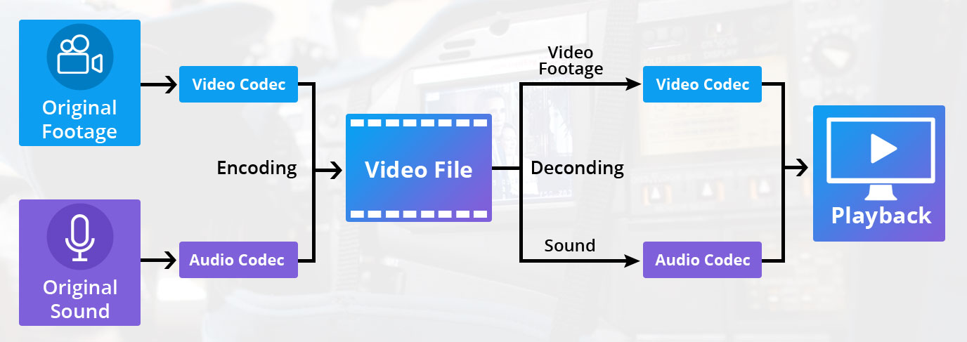
As people directly related to the AV sphere, we constantly talk about audio coding and audio codecs, but what is it? An audio codec is essentially a device or algorithm that can encode and decode a digital audio signal.

In practice, the audio waves that travel through the air are continuous analog signals. The signals are converted to digital form by a device called an analog-to-digital converter (ADC), and the reverse converter is called a digital-to-analog converter (DAC). The codec lies between these two functions and it is he who allows you to adjust some important parameters for the successful capture, recording and transmission of an audio signal: the codec algorithm, the sampling frequency, the bit width and the speed of the audio signal. data.

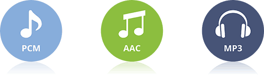
The three most popular audio codecs are Pulse-Code Modulation (PCM), MP3, and Advanced Audio Coding (AAC). The choice of codec determines the compression rate and the recording quality. PCM is a codec used by computers, CDs, digital phones, and sometimes SACD. The PCM signal source is sampled at regular intervals, and each sample is the digital amplitude of the analog signal. PCM is the simplest option for digitizing an analog signal.

With the correct parameters, this digitized signal can be completely converted back to analog without any loss. But this codec, which provides an almost complete identity with the original audio, is unfortunately not very cheap, which results in very large file sizes, and such files are not suitable for streaming. We recommend using PCM to record digital images for your sources or when doing audio post-processing.

Fortunately, we always have the option of choosing a different codec that can compress digital data (rather than PCM) based on some helpful observations on the behavior of sound waves. But in this case, you have to make a compromise: all alternative algorithms are associated with “losses”, since it is impossible to completely restore the original signal, but nevertheless the result is still so good that most users will not be able to to catch the difference.

MP3 is an audio encoding format that uses a digital data compression algorithm that allows you to save the audio signal in smaller files. The MP3 codec is the most used by users to record and store music files. We recommend using MP3 to stream audio content as it requires less network bandwidth.

AAC is a newer audio encoding algorithm that is the successor to MP3. AAC has become the standard for the MPEG-2 and MPEG-4 formats. In fact, this is also a digital data compression codec, but with less quality loss than MP3 when encoded with the same bit rate. We recommend using this codec for online streaming.

Digital audio encoding

Digital audio encoding

Digital audio encoding

PC-based audio coding is based on the process of converting air vibrations into electrical current fluctuations and the subsequent sampling of an analog electrical signal.

DIGITAL AUDIO ENCODING

The encoding and reproduction of audio information is carried out using special programs. The quality of reproduction of the encoded sound depends on the sampling frequency and its resolution (sound encoding depth – the number of levels).

Digital audio is an analog audio signal represented by discrete numerical values of its amplitude.

Sound digitization is a technology with a divided time step and subsequent recording of the values obtained in numerical form. Another name for digitizing audio is analog to digital audio conversion, which includes the following operations:

Bandwidth limiting is done by using a low pass filter to suppress spectral components that are more than half the sample rate.

Time sampling, that is, replacing a continuous analog signal with a sequence of its values at discrete moments of time: samples.

Level quantization is the replacement of the signal’s reference value with the closest value of a set of fixed values: quantization levels.

Encoding or digitization, as a result of which the value of each quantized sample is represented as a number corresponding to the ordinal number of the quantization level.

This is done as follows: a continuous analog signal is “cut” into sections with a sample rate, a discrete digital signal is obtained, which goes through the quantization process with a certain bit depth, and is then encoded, that is, it is replaced by a sequence of code symbols. To record sound in a 20-20,000 Hz frequency band, a sampling frequency of 44.1 and higher is required (today there are ADCs and DACs with a sampling frequency of 192 and even 384 kHz). To obtain a high-quality recording, 16-bit is sufficient, however, to expand the dynamic range and improve the quality of the sound recording, 24 (less often 32) bits are used.

Sound coding methods (of course an electrical signal coming from a microphone) are based on the fact that, theoretically, any complex sound can be decomposed into a sequence of simpler harmonic signals of different frequencies, each of which it is a sinusoid, called the spectrum of the original signal. The task of encoding sound, like any other analog signal, is to represent it in the form of another analog or digital signal, which is more convenient for its transmission or storage in each specific case. Real sound sources have a limited spectrum width, therefore, for encoding, transformation methods are used that transform the original signal into one, the spectrum of which is more suitable for transmission on the selected channel. Representing an analog signal as another analog signal is commonly referred to as modulation and digitally as encoding. This division is very arbitrary. An analog signal can be represented as a harmonic signal (that is, a sinusoid), the parameters of which change depending on the value of the original signal. In the event that the amplitude of the sinusoid changes with a change in the original signal, it is amplitude modulation (AM). If, depending on the value of the original signal, the frequency or phase of the sinusoid changes, we are dealing with frequency modulation (FM) or phase modulation (PM). Amplitude and frequency modulation, for example, is widely used to transmit sound by radio. These types of modulation, of course, are not the decomposition of the original signal into harmonics. The development of digital technology and the use of computer processing and information storage has led to the widespread use of pulse encoding or modulation methods. Such types of modulation are, for example, pulse code modulation, in which the value of the original signal at regular intervals is represented in code form. The vast majority of “computer sound” is precisely the recording of the binary code of the received signal in short equal time intervals, determined by the sampling frequency. For storage and transmission through communication channels, this signal is usually compressed (reducing the volume by discarding unnecessary or insignificant information). In addition to pulse code modulation, other types of digital modulation (pulse width, pulse frequency, etc.) are also used to encode sound.

Audio encoding.

Audio encoding.

AUDIO ENCODING

Digital audio is an analog audio signal represented by discrete numerical values of its amplitude.

audio encodig

Sound digitization is a technology with a divided time step and subsequent recording of the values obtained in numerical form.

Another name for digitizing audio is analog to digital audio conversion.

Sound digitization involves two processes:

sample (sample) a signal over time
amplitude quantification process.
Meanwhile, there is no need to worry about it. ”

Discretization of time.

Meanwhile, there is no need to worry about it. ”

The time sampling process is the process of obtaining the values of the signal that is being converted, with a certain time step: the sampling step. The number of measurements of the magnitude of the signal, carried out in one second, is called the sampling frequency or the sampling rate, or sampling frequency (from the English “sampling” – “sampling”). The lower the sampling step, the higher the sampling frequency and the more accurate representation of the signal that we will obtain.

This is confirmed by Kotelnikov’s theorem (in foreign literature it is found as Shannon’s theorem, Shannon). According to him, an analog signal with a limited spectrum can be accurately described by a discrete sequence of values of its amplitude, if these values are taken with a frequency that is at least twice the highest frequency in the spectrum of the signal. That is, an analog signal in which the highest spectrum frequency is F m can be accurately represented by a sequence of discrete amplitude values if F d> 2F m is satisfied for the sampling frequency F d.

In practice, this means that for the digitized signal to contain information on the full audible frequency range of the original analog signal (0 – 20 kHz), it is necessary that the selected sample rate be at least 40 kHz. The number of amplitude measurements per second is called the sampling rate (if the sampling step is constant).

The main difficulty of digitization is the inability to record the measured signal values with perfect precision.

Analog to digital converters (ADC).

Meanwhile, there is no need to worry about it. ”

The above process of digitizing sound is done using analog-to-digital converters (ADCs).

This transformation includes the following operations:

Bandwidth limiting is done by a low pass filter to suppress spectral components that are more than half the sample rate.
Discretization in time, that is, substitution of a continuous analog signal with a sequence of its values at discrete moments in time: samples. This problem is solved by using a special circuit at the input of the ADC – a sample and hold device.
Level quantization is the replacement of the signal’s reference value with the closest value of a set of fixed values: quantization levels.
Encoding or digitization, as a result of which the value of each quantized sample is represented as a number corresponding to the ordinal number of the quantization level.
This is done as follows: a continuous analog signal is “cut” into sections with a sample rate, a discrete digital signal is obtained, which goes through a quantization process with a certain bit depth, and is then encoded, that is, it is replaced by a sequence of code symbols. To record sound in a frequency band of 20-20,000 Hz, a sampling frequency of 44.1 and higher is required (today there are ADCs and DACs with a sampling frequency of 192 and even 384 kHz). To obtain a high-quality recording, 16 bits are sufficient, however, to expand the dynamic range and improve the quality of sound recording, 24 (less often 32) bits are used.

Meanwhile, there is no need to worry about it. ”

Encoding methods.

Frequency modulation.

Sound coding methods (of course we mean the electrical signal coming from the microphone) are based on the fact that, in theory, any complex sound can be broken down into a sequence of the simplest harmonic signals of different frequencies, each one of which is a sinusoid, called the original signal spectrum. The task of encoding sound, like any other analog signal, is to represent it in the form of another analog or digital signal, more convenient for its transmission or storage in each specific case.

Audio encoding and processing.

Audio encoding and processing.

Parameters that affect digital sound quality Minimum and maximum sound quality.

Audio encoding and processing

My grandfather was listening to a gramophone. My father’s youth turned to music coming from the speaker of a reel-to-reel tape recorder. The heyday and decline of cassette recorders fell upon my youth. My son is growing up in the age of digital audio. To keep up to date and give my son a good “sound”, I decided to find out what determines the quality of the digital audio signal reproduction.

I talked to my music loving friends. He did an information search on the Internet. As a result, I came to the conclusion that high-quality sound can be achieved in the digital age by choosing the right 7 basic elements of modern music centers:

the format in which the music is recorded;
player;
digital to analog converter;
amplifier;
acoustics;
cables;
food.

Below I will share my observations and conclusions on achieving high quality sound recordings in digital formats.

Lyrical digression, experts don’t need to read.

In a nutshell, I will explain where digital sound comes from. During the recording process, the microphone converts mechanical vibrations (the sound itself) into an analog electrical signal. An analog signal is, in the most general case, similar to a sinusoid that has been familiar to all of us since high school. In the age of analog sound, it was this signal that was recorded on various media and then played back.

With the development of microprocessor technology, it became possible to record and store audio information in digital formats. These formats are obtained through an analog-to-digital conversion (ADC) process.

During the ADC, the analog signal (our high school sine wave) becomes a discrete one (in other words, it is cut into pieces). In the next stage, the discrete signal is quantized, that is, each resulting segment of the sinusoid is assigned a digital value. In the third step, the quantized signal is digitized, ie encoded in the form of a sequence of 0 and 1. With respect to digital sound recording, the information about the amplitude and frequency of the sound is digitized.

To record and store digital audio information, digital audio formats are used. The audio format is understood as a set of requirements for the digital representation of audio data.

When it comes to sound quality, digital formats are divided into 3 categories:

Formats without additional compression (CDDA, DSD, WAV, AIFF, etc.);
Lossless compressed formats (FLAC, WavPack, ADX, etc.);
Lossy compression formats (MP3, AAC, RealAudio, etc.).

High-quality sound is obtained when playing music saved in formats of the first and second category. In the formats of the third category, to reduce the amount of data, part of the information is deliberately excluded. For example, information about hidden frequencies.

Latent frequencies are those that are outside the range of perception of the average person: 20 Hz – 22 kHz. For audiophiles, this range is wider due to individual psychophysiological characteristics.

To complete your home audio library, you must select records saved in files with the following extensions:

* .wav, * .dff, * .dsf, * .aif, * .aiff are uncompressed sound files;
* .mp4, * .flac, * .ape, * .wma are the most common lossless compressed audio files.
From history. They say that the first experiments on the preservation of sound were carried out by the ancient Greeks. They tried to keep the sound in amphorae. It looked something like this: words were spoken into the amphora and it was quickly sealed. Unfortunately, none of those records have survived to this day.