Lossy Compression Part 2


Free Download Mp4Gain
picture

Lossy Compression Part 2
Lossy Compression

Compress audio and video

LOSSY COMPRESSION

The term “bit rate” refers to the number of bits of information transmitted per second. This term is translated into Russian in different ways in different sources. Recently, the word “bitrate”, which is new to the Russian language, is often used instead of a formal translation. The translation options are also as follows: “data stream width”, “bit stream complexity”, “stream rate”, “bit rate”. This same parameter is sometimes called the file compression rate for sound files. For example, the file is said to be compressed at 128 Kbps. The fact is that the bit rate value is directly related to the physical size of the sound file per second of sound.

All compression formats of the MPEG family use a high redundancy of information in images separated by a short time interval. Between two adjacent frames, usually only a small part of the scene changes; for example, there is a smooth movement of a small object against the background of a fixed background. In this case, the complete information about the scene is saved selectively, only for reference images. For the rest of the frames, it is enough to transmit differential information: on the position of the object, the direction and magnitude of its displacement, on new background elements that open up behind the object as it moves. Furthermore, these differences can form not only in comparison with the previous images, but also with the later ones (since it is in them, as the object moves, that the previously hidden part of the background is revealed).

The MPEG family of compression formats reduces the amount of information as follows:

Temporal video redundancy is eliminated (only difference information is considered).
The spatial redundancy of the images is eliminated by suppressing the small details of the scene.
Some of the color information is removed.
The information density of the resulting digital stream is increased by choosing the optimal mathematical code for its description.
MPEG compression formats compress only anchor frames: I-frames (intraframes). The intervals between them include frames that contain only changes between two adjacent I-frames: P-frames (predicted frame – predicted frame). To reduce the loss of information between the I frame and the P frame, so-called B frames (bidirectional frame) are introduced. They contain information that is taken from the previous and next frames. When encoding in MPEG compression formats, a chain of frames of different types is formed. A typical sequence of frames looks like this:

I B B P B B I B B P B B I B B …

Consequently, the sequence of frames according to their numbers will be played in the following order:
1 4 2 3 7 6 5 …


Free Download Mp4Gain
picture


Mp4Gain Main Window
picture


Mp4Gain Features
picture


Free Download Mp4Gain
picture

Lossy compression

Lossy compression

Lossy compression

Compress audio and video

lossy compression

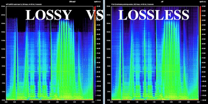
High-quality digitized audio requires a large amount of disk space. Attempts to reduce file sizes using standard cabinets do not yield significant gains due to the specificity of the audio data. However, it is possible to achieve a fairly significant level of compression of the audio information using special methods based on the analysis of the data structure and subsequent compression with some loss.

The real possibility of sound processing comparable in quality to existing analog examples appeared only in the late 1980s. In 1988, the International Organization for Standardization (ISO) formed the MPEG (Moving Pictures Expert Group) committee, whose main task is develop coding standards for moving images, sound and their combination. During the ten years of its existence, the committee has developed a series of norms on this subject. As a result, when summarizing extensive research in this area, several specific formats were recommended for storing data, differing in the quality of the results and the data flow.

Currently, there are three most common video storage standards: MPEG-1, MPEG-2, and MPEG-4. Within the first two formats, there are also formats for storing audio information: Layer-1, Layer-2 and Layer-3. These three audio formats are defined for MPEG-1 and minor extensions are used in MPEG-2. The three formats are similar to each other, but use different levels of compression and complexity compensation. Layer-1 is the simplest, it does not require significant compression costs, but it also provides a negligible compression ratio. Layer-3 level: the most time consuming and provides the best compression. Recently, this format has gained immense popularity. It is often called MP3. This name is associated with the extension of the audio files stored in this format.

Founded idea, in which all lossy audio signal compression methods – ignore the subtle details of the original sound, which are outside of that perceived by the human ear. Here several points can be highlighted.

Noise level. Sound compression is based on a simple fact: if a person is next to a loud siren, it is unlikely that he will hear the conversation of the people who are nearby. Also, this happens not because a person pays close attention to a loud sound, but to a greater extent because the human ear actually misses out sounds that are in the same frequency range as a louder sound. This effect is called masking, it changes with the difference in volume and frequency of the sound.

The second point is the division of the audio frequency band into subbands, each of which is further processed separately. The encoding program extracts the loudest sounds from each band and uses this information to determine an acceptable noise level for that band. The best encoding programs also take into account the influence of adjacent bands. A very loud sound in one band can affect the masking effect and nearby bands.

Another point of coding is the use of a psychoacoustic model based on the peculiarities of human perception of sound. Compression The use of this model is based on the removal of obviously inaudible frequencies with a more careful preservation of sounds that are clearly distinguishable by the human ear. Unfortunately, there can be no exact mathematical formulas here. Human perception of sound is a complex process that is not fully understood, so the choice of compression methods is based on analyzing listening and comparing compressed sounds differently by teams of experts. But here there are practically unlimited possibilities in the field of improving psychoacoustic models. Most of the existing algorithms to encode the human voice are based on the high predictability of said signal; Universal MPEG compression algorithms have tried to apply this technique with variable success.

Lossless Audio Compression Part 3

Lossless Audio Compression Part 3

Lossless Audio compression

An overview of the most common audio codecs.

lossless audio

DVD Audio adopts the MLP lossless data compression algorithm developed by Meridian. And SACD is used, unlike other formats. Three ways to encode audio. Macromedia Flash Professional 8. We study both formats with lossless compression and lossy compression of mp3 and the like, based on human quirks. AllFrets audio file formats. Inverse Fourier transform for real sounds without loss of quality of psychoacoustics used in lossy audio compression algorithms. Lossy Audio – Lossy Format – What You Need To Know. Lossless compression from a perceptual point of view. Facts Well, in terms of sound, nothing better than the old and well-known MP3 has been invented. Then. Methods of compression of images, audio signals and educational video. The lossless compression algorithm for integer data, the Salomon D values, is considered.

Lossless Audio Compression Knowledge Map.
Lossless Audio Converter converts from one lossless audio compression format to another. FLAC, ALAC, WMA Lossless, WAV, APE are supported. Lossless audio codec TTA Compression theory Tau projects. The most common lossless compression formats are: Free Lossless Audio Codec FLAC, Apple Lossless, MPEG 4 ALS ,. Multimedia technologies in CAD. Part II: Tutorial. Powerful lossless compression algorithm. A rare branch of this type of algorithm. Lossless audio encoding zi p. A brief description is given. Understand lossless audio conversion and decompression. There are two main types of compression: lossless compression and lossy compression. The most famous compression format is c.

Recommendations for using the mp3 compression standard.
Examples of lossy and lossless compression algorithms and data formats are given for transferring text, audio and video information. Text. Audio compression format MP3 Helpix.Org. Remember that along with digital sound there is analog sound or graphic files, the audio signal cannot be compressed without loss of compression based on removing unnecessary sounds from the music file.

Lossless audio compression.
A set of transformations that efficiently compress the audio data with the possibility of full recovery.  The block statistics for each data block are calculated separately and added to the most compressed block. Lossless audio compression C. Lossless data compression eng. Lossless data compression is a class of data compression algorithms for video, audio, graphics, and documents presented in.

Useful Information Lossless formats for Cinetec kettles.
Free Lossless Audio Codec Free Lossless Audio Codec is a popular free codec for audio compression. Unlike lossy codecs. Sound compression life prog. This method is the opposite of lossless audio compression used for formats like FLAC, ALAC, and others.

Files with Hi Fi sound.
What are the ways to store lossless audio? Which lossy compression format is better to use: mp3, LQT, WMA, MP, ogg vorbis…. Lossless information compression. First part Habr Habr. Lossless: FLAC, ALAC, WAV Lossy: MP3, AAC, OGG, WMA. Compressed audio storage formats: MP3, AAC, OGG and others. Lossless format what is it? High quality music c. Lossless Audio Compression A set of transforms that allow you to compress efficiently. Visit the site for more information. Is there a difference between MP3, AAC, FLAC and. Lossless audio files are usually larger, the definition of the concept is derived from the name – uncompressed raw data.

Digital Audio Compression Methods from the Academy of Digital Music.
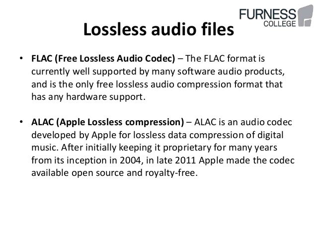
FLAC is possibly the most popular lossless audio compression format. FLAC. FLAC format. Free lossless audio codec. LossyWAV. Audio compression: 6.4. Well established methods. Lossy compression is mainly used for JPEG graphics, MP3 audio, MPEG video, that is, where, due to the huge file sizes, the degree.

Lossless audio compression Part 2

Lossless audio compression Part 2

lossless audio compression

The moderate compression ratio of a standard 4: 1 audio signal allows multiple sound encodings and decodes without noticeable loss of quality. Edition

LossLess

and frequency. The amplitude characterizes the volume of the sound. The frequency determines the pitch, the pitch cm. The pitch of sound An ordinary person can hear the vibrations of sound
HDTV broadcasts, where it is encoded by Dolby Digital and DTS lossy compression systems, and DTS HD Master Audio and Dolby TrueHD lossless audio compression formats in HDTV broadcasts
of encoded sound depends on sample rate and resolution sound encoding depth – number of levels Portal Digital sound Digital sound is
free encoders: Speex – for voice compression FLAC – for lossless audio compression Theora – for video compression. Vorbis uses the container format to store sound
mainly speaks. TTA – Lossless Compression Vorbis – Lossy Compression developed by Xiph.org. WavPack – Lossless Lossy Compression from MPEG Licensing Authority
recovery of losses caused by interference during transmission, as well as in other applications. Digital audio is a technology for converting analog audio to digital.
To reduce the transmission bandwidth required for DSD, lossless audio compression DST eng. Direct Stream Transfer DST standardized in 2005
4720 and 4720 respectively. AMR was also widely used for audio compression when recording video in 3GPP format on mobile phones. There is a free.

Why is the operation of compressing audio information performed?
Lossless compression. This encoding method is used in almost all lossless HRA codecs, which have a minimum frequency. Lossy audio compression. Compression of AlgoList audio signals. It provides a not very strong compression, but without losses. It is currently only used to compress very short audio clips, mostly.

What is the principle of file compression?

We managed to easily compress the directory with WAV tracks with a total size of 406. For lossless sound compression, you can use. Lossless compression Lossless Theory Sound characteristics. Lossless compression. Compression techniques or lossless compression algorithms can be classified according to the type of data they were for.

Lossless audio compression

Lossless audio compression

 lossless

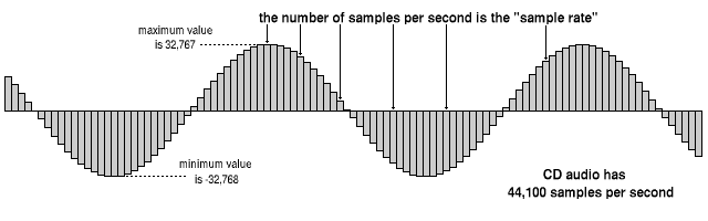
Sound is a simple wave and digitized sound is a digital representation of that wave.

LOSSLESS AUDIO COMPRESSION

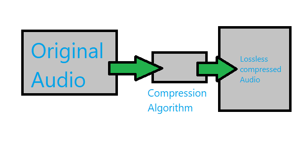
This is accomplished by storing the level of the analog signal several times in one second. For example, on an ordinary CD, a signal is stored 44100 times per second. Since the CD works with stereo, we store the signal for the left and right speakers in parallel. 16-bit numbers are used for each measurement. So it’s easy to calculate that one second of polling takes 2 × 2 × 44100 = 176,400 bytes. Lossless audio compression is a set of transformations that efficiently compress the audio data with the possibility of its complete recovery. Like any lossless compression, audio data compression exploits some characteristic of the data. In this case, these are:
Knowing the limits of the samples: We know how many bits or bytes are allocated per sample sample and how many audio channels are in the sample.
Low derivative: In other words, the values ​​of the adjacent samples differ little.
Low second derivative: the values ​​of the three adjacent samples are close to a linear function.
Closeness of the left and right channels: The signal levels in the left and right speakers are usually close.

Rice’s algorithm
The idea behind audio compression is to represent the numbers corresponding to the stream as small as possible, removing any data correlation beforehand. You can then write the encoded data stream to disk. One of the most efficient ways is Rice encoding. Smaller numbers are preferred because their binary representation is shorter. For example, you need to encode the following row: Base in base 10:10, 14, 15, 46 OR the same row in binary form Base 2: 1010, 1110, 1111, 101110 Now if you want to represent this as a string, where 32 bits are reserved for each number for the range of all possible values, it will be ineffective, since 128 bits are needed. However, there is a more effective method. The best solution would be to simply write the binary numbers 1010, 1110, 1111, 101110 without commas, obtaining a series like 101011101111101110. The problem is that afterwards there is no way to know the limits of each number. As a general rule, the Rice algorithm is used as a solution to this problem. Rice encoding is a way of representing small numbers on a single line while still being able to distinguish them. Note: the smaller the numbers, the more efficient the algorithm will be, so you need to deal with this initially. At some stage in encoding, the data is represented as a number n. When encoded, it is added to the right of the string of already encoded numbers in such a way that the reverse process is possible. The basic idea is to represent the number n as n = q ∗ 2 k + r {\ displaystyle n = q * 2 ^ {k} + r} so that 0

MP3 bitrate types

MP3 bitrate types

Mp3 Bitrate

Bit rate

bitrate

CBR stands for constant bit rate, that is, a constant bit rate that is set by the user and does not change when the part is encoded. Therefore, every second of the part corresponds to the same number of bits of encoded data (even when encoding silence).

VBR stands for variable bit rate, that is, a variable bit rate or variable bit rate that the encoder program dynamically changes during encoding based on the saturation of the audio material being encoded and the encoding quality set by the user (for example, silence is encoded with the minimum bit rate). The downside to this encoding method is that VBR considers the quietest snippets to be “negligible” audio information, so it turns out that if you listen too loud, these snippets will be of poor quality, while CBR makes quiet and loud snippets with the same bit rate …

ABR stands for Average Bit Rate, that is, Average Bit Rate, which is a hybrid of VBR and CBR: the user sets the bit rate in kbit / s and the program varies it, constantly adjusting it to the specified bit. Velocity. Therefore, the codec will be careful to use the maximum and minimum possible bitrate values, as it runs the risk of not conforming to the bitrate specified by the user. This is a clear disadvantage of this method, as it affects the quality of the output file, which will be slightly better than using CBR, but worse than using VBR (with the same file size).

MP3 codecs

The type of programs required to convert file formats. The most common MP3 codecs are:

mp3PRO-codec (uses SBR frequency transform).
LAME codec
fraunhofer-codec

Digital audio compression methods

Digital audio compression methods

audio compression

Lossless compression

AUDIO COMPRESSION

Generally speaking, the meaning of lossless compression is as follows: some pattern is found in the original data, and taking this pattern into account, a second stream is generated, uniquely describing the original. For example, to encode binary sequences in which there are many zeros and few ones, we can use the following replacement:

00> 0
01> 10
10> 110
11> 111

In this case, sixteen bits:
00 01 00 00 11 10 00 00

will be converted to thirteen bits:
0 10 0 0 111 110 0 0

If we write a compressed string without spaces, we can still add spaces in it, which means restoring the original sequence.

FLAC (Free Lossless Audio Codec)
Coding principle: the algorithm tries to describe the signal with this function so that the result obtained after subtracting it from the original (called difference, remainder, error) can be encoded with the minimum number of bits.

When the model is fitted, the algorithm subtracts the approximation from the original to obtain a residual signal (error), which is then losslessly encoded.

Lossy compression (MP3, AAC, WMA, OGG)
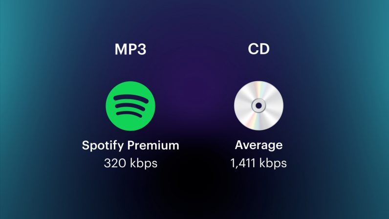
Using a lossy compression algorithm, the size of an MP3 file with an average bit rate of 128 kbps is approximately 1/11 of the original file of an Audio CD (uncompressed audio in CD-Audio format has a rate bit rate of 1411.2 kbps). MP3 files can be created at high or low bit rates, which affects the quality of the result.

The principle of compression is to reduce the precision of some parts of the sound flow, which is almost indistinguishable for most people. The audio signal is divided into segments of equal length, each of which, after processing, is packed into its own frame (frame). Spectral decomposition requires continuity of the input signal; therefore the table above and below are also used for calculations. The audio signal contains harmonics with a lower amplitude and harmonics that are close to the strongest; Such harmonics are cut off, as the average human ear will not always be able to determine the presence or absence of such harmonics. This characteristic of hearing is called the masking effect. It is also possible to replace two or more nearby peaks with an averaged one (which, as a rule, leads to sound distortion). The cutoff criterion is determined by the outflow requirement. Since the entire spectrum is relevant, the high-frequency harmonics are not cut off, but are only selectively removed to reduce information flow due to spectrum sparsity. After spectral removal, mathematical compression and frame packing methods are applied.

Masking effect
In certain cases, a sound can be hidden by another sound. For example, talking near the railroad tracks can be completely impossible if a train passes. This type of effect is called masking. A weak sound is said to be masked if it becomes indistinguishable in the presence of a louder sound.

Simultaneous masking
Any two sounds when heard simultaneously have an impact on the perception of the relative volume between them. A louder sound reduces the perception of a weaker one, until the disappearance of your hearing. The closer the frequency of the masked sound is to the frequency of the masker, the more it will be hidden. The masking effect is not the same when the masked sound is shifted down or up in frequency with respect to masking. Low-frequency sound masks high-frequency sound. However, it is important to note that high-frequency sounds cannot mask low-frequency sounds.

Time masking
This phenomenon is similar to frequency masking, but time masking occurs here. When the masking sound is stopped, the masking remains inaudible for some time. Under normal conditions, the temporary masking effect lasts significantly less. The masking time depends on the frequency and amplitude of the signal and can be up to 100 ms.
In the case where the masking tone appears at a time after masking, the effect is called post-masking. When the masking tone appears before the masking (this is also possible), the effect is called premasking.

Post-stimulus fatigue
Often after exposure to loud, high-intensity sounds, a person’s hearing sensitivity drops dramatically. Recovery to normal thresholds can take up to 16 hours. This process is called “temporary change in hearing sensitivity threshold” or “post-stimulus fatigue.”

Bits, Hertz, Shaped Dithering … Part 3

Bits, Hertz, Shaped Dithering … Part 3

bits

What is behind these concepts?

BITS

For transmission of sound as is, it would be nice to keep the entire perceived range from 10 Hz to 20 kHz. In theory, there is absolutely no problem with low frequencies in digital recording (but there are problems with transmitting these frequencies through electrical circuits and reproducing them through small stereo speakers or headphones). So, at the output of the sound cards there is usually a power amplifier, which feeds the signal to the stereo speakers. This inexpensive board amplifier, together with the feedback circuit, as well as the parasitic capacitances, forms a low pass filter that “dumps the bass.”

With high frequencies, things are a bit worse, at least definitely more complicated. Most of the essence of the DAC and ADC enhancements and complications is aimed precisely at more reliable transmission of high frequencies. “High” means frequencies comparable to the sampling frequency, that is, in the case of 44.1 kHz, it is 7 to 10 kHz and more.

Imagine a 14 kHz sinusoidal signal digitized at a 44.1 kHz sample rate. There are about three points (samples) for one period of the input sinusoid, and to restore the original frequency as a sinusoid, you need to show some imagination. The sample waveform restoration process also occurs in the DAC, this is done using the restoration filter. And if the relatively low frequencies are almost pre-cast sinusoids, then the shape and consequently the quality of the reconstruction of the high frequencies is completely dependent on the conscience of the DAC restoration system. Therefore, the closer the signal frequency is to one-half the sampling frequency, the more difficult it is to reconstruct the shape of the signal.

This is the main problem when it comes to reproducing high frequencies. However, the problem is not as serious as it might seem. All modern DACs use resampling (multi-rate) technology, which involves restoring digitally to a sample rate several times higher and then converting it to an analog signal at an increased rate. Thus, the problem of restoring high frequencies shifts to the shoulders of digital filters, which can be of very high quality. So high quality that in the case of expensive devices the problem is completely eliminated: distortion-free reproduction of frequencies up to 19-20 kHz is provided. Resampling is also used in inexpensive devices, so this problem can be considered solved in principle. Devices in the region of $ 30- $ 60 (sound cards) or stereos up to $ 600, generally similar in DAC to these sound cards, perfectly reproduce frequencies up to 10 kHz, tolerably up to 14-15, and somewhat way the rest. This is sufficient for most real music applications, and if someone needs more quality, they will find it in professional quality devices, which are not much more expensive, they are simply made with the mind.

Bits, Hertz, Shaped Dithering … Part 2

Bits, Hertz, Shaped Dithering … Part 2

bits

What is behind these concepts?

Bits

In theory, this is the only criterion for choosing the scanning resolution. We no longer contribute absolutely without distortions or inaccuracies. The practice, oddly enough, almost completely repeats the theory. This is what guided those people who chose 16-bit resolution for audio CDs. Noise of minus 93 decibels is a pretty good condition, which corresponds almost exactly to the conditions of our perception: the difference between the pain threshold (140 decibels) and the usual background noise in the city (30-50 decibels) is of about a hundred decibels, and if we consider that the painful volume level, no music is heard, which further reduces the range, it turns out that the actual noise from the room or even from the equipment is much louder than the noise from quantification. If we can hear a level below minus 90 decibels in a digital recording, we will hear and perceive quantization noises; otherwise we will simply never determine whether it is live or digital audio. There is simply no other difference in terms of dynamic range. But, in principle, a person can hear significantly in the 120 decibel range, and it would be nice to keep this full range, which apparently 16 bits cannot support.

But this is only at first glance: using a special technique called shape dithering, it is possible to change the frequency spectrum of the sampling noise, bringing them almost completely into the region of more than 7-15 kHz. In a way, we changed the resolution of the frequency (we refused to reproduce quiet high frequencies) to get additional dynamic range in the remaining frequency segment. In combination with the peculiarities of our hearing, our sensitivity to the ejected high-frequency region is tens of dB lower than in the main region (2-4 kHz), this makes possible a relatively quiet transmission of useful signals by 10-20 additional dB quieter than -93 dB; therefore, the dynamic range of human 16-bit audio is approximately 110 decibels. And in general, at the same time, a person simply cannot hear sounds 110 decibels lower than the loud sound that he just heard. The ear, like the eye, adjusts to the volume of the surrounding reality, therefore the simultaneous range of our hearing is relatively small, around 80 decibels. Let’s talk more about dithring after discussing the frequency aspects.

For CD, the sampling frequency is 44100 Hz. There is an opinion (based on a misunderstanding of the Kotelnikov-Nyquist theorem) that all frequencies are reproduced up to 22.05 kHz, but this is not entirely true. We can only say that there are no frequencies above 22.05 kHz in the digitized signal. The actual image of digitized sound reproduction always depends on the specific technique and is not always as ideal as we would like, and as befits the theory. It all depends on the specific DAC (digital to analog converter responsible for receiving an audio signal from a digital stream).

Let’s first find out what we would like to achieve. A middle-aged (quite young) person can feel sounds from 10 Hz to 20 kHz, hear significantly – from 30 Hz to 16 kHz. The loudest and lowest sounds are heard, but are not acoustic sensations. Sounds above 16 kHz are felt as an annoying and unpleasant factor: pressure on the head, pain, especially loud sounds, cause such acute discomfort that one wants to leave the room. The unpleasant sensations are so strong that the action of the security devices is based on this: a few minutes of very loud high-frequency sound will drive anyone crazy and it becomes absolutely impossible to steal anything in such an environment. Sounds below 30 – 40 Hz with sufficient amplitude are perceived as vibrations emanating from objects (speakers). It would be more correct to say, just vibration.

Bits, hertz, shaped dithering …

Bits, hertz, shaped dithering …

bits

What is behind these concepts?

bits

When developing the standard for CD Audio (CD Audio), 44 kHz, 16-bit, and 2-channel (ie stereo) settings were adopted. Why exactly so many? What is the reason for this choice, and also why are attempts being made to increase these values ​​to, say, 96 kHz and 24 or even 32 bits …

Let’s first find out with the sampling resolution, that is, with the bitness. You happen to have to choose between the numbers 16, 24 and 32. The middle values ​​would of course be more convenient in terms of sound, but too unpleasant for use in digital technology (a very controversial statement, since that many ADCs have 11 or 12 bit digital output (status approx.).

What is this parameter responsible for? Simply put, for dynamic range. The volume range played simultaneously is from the maximum amplitude (0 decibels) to the lowest that the resolution can transmit, for example, approximately minus 93 decibels for 16-bit audio. Interestingly, this is strongly related to the noise level of the soundtrack. In principle, for 16-bit audio, it is quite possible to transmit signals with a power of -120 dB, however, these signals will be difficult to apply in practice due to such a fundamental concept as sampling noise …. The fact is that when taking digital values, we always make mistakes, rounding the true analog value to the closest possible digital value. The smallest possible error is zero, but at most we are wrong with half of the last bit (bit, hereinafter, the term least significant bit will be abbreviated MB). This error gives us the so-called sampling noise, a random discrepancy between the digitized signal and the original. This noise is constant and has a maximum amplitude equal to half of the least significant bit. This can be considered as random values ​​mixed in the digital signal. This is sometimes called rounding noise or quantization noise (which is a more accurate name since encoding the amplitude is called quantization, and sampling is the process of converting a continuous signal into a discrete sequence (pulses) – approx . comp.).

Let’s dwell in more detail on what is meant by signal power, measured in bits. The strongest signal in digital audio processing is generally taken as 0 dB, this corresponds to all bits set to 1. If the most significant bit (hereinafter SB) is set to zero, the resulting digital value will be half, which corresponds to a loss level of 6 decibels (10 * log (2) = 6). Therefore, by zeroing the most significant bits to the least significant, we will decrease the signal level by six decibels. It is clear that the minimum signal level (one in the least significant bit and all other digits are zeros) is (N-1) * 6 dB, where N is the digit capacity of the sample. For 16 digits, the weakest signal level is 90 decibels.

When we say “half the least significant bit”, we do not mean -90/2, but half a step to the next bit, that is, another 3 decibels less, minus 93 decibels.

We return to the choice of scanning resolution. As already mentioned, digitization introduces noise at the level of the middle of the least significant bit, which means that a 16-bit digitized record constantly makes noise at minus 93 decibels. It can transmit signals and is quieter, but the noise is still -93 dB. On this basis, the dynamic range of digital sound is determined: where the signal-to-noise ratio is transformed into noise / signal (there is more noise than the useful signal), the edge of this range is at the bottom. Therefore, the main criterion for digitizing is the amount of noise. Can we afford a recovered signal? The answer to this question depends in part on how much noise was on the original track. An important conclusion: if we digitize something with a noise level of less than 80 decibels, there is absolutely no reason to digitize it to more than 16 bits, since, for one thing, the noise of -93 dB adds very little to the existing one. Huge (comparatively) noise of -80 dB and, on the other hand, quieter than -80 dB on the phonogram itself, the noise / signal already starts, and there is simply no need to digitize and transmit said signal.