Digital audio compression

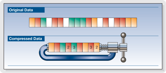
Audio data compression is a real problem today. There are two reasons for the need to compress audio data: memory savings when storing audio information, low bandwidth of remote digital information transmission channels. Compression effectively solves the two problems above. Data compression is an algorithmic transformation of data performed to reduce its volume.

It is used for a more rational use of data storage and transmission devices. Compression is based on eliminating the redundancy contained in the original data. To guarantee the parameters necessary for the transmission of voice signals (music) over modern low-speed digital communication channels and to guarantee the specified noise immunity, it is necessary to use highly efficient data compression algorithms. The transmission channel is characterized by a concept such as the capacity of the channel: And the signal – by the volume (signal): …
Both of the above features include dynamic range D, channel width (signal spectrum), and transit time T. Digital audio compressors are used to reduce dynamic range. To improve spectral efficiency, digital filters are used to limit the spectrum of the encoder output signal (according to Nyquist criteria). Among other things, encoders based on the principles of elimination of redundancy (Huffman codes) are used to guarantee a certain information transmission speed. The essence of which is as follows: codes based on the principle of assigning more probable values of the amplitudes of the codewords of shorter length than the improbable ones.
Let’s consider how the types of redundancy described above are eliminated.
Structure of a lossy audio compression encoder The original digital audio signal is divided into frequency subbands and time-segmented into a time-frequency segmentation block. The length of the encoded sample depends on the shape of the temporal function of the audio signal. In the absence of sharp peaks in amplitude, a long sample is used, which provides high-frequency resolution. In the case of abrupt changes in signal amplitude, the length of the encoded sample decreases dramatically, giving a higher time resolution. The decision to change the length of the coded sample is made by the psychoacoustic analysis unit, calculating the value of the psychoacoustic entropy of the signal.
After segmentation, the frequency subband signals are normalized, quantized, and encoded. In the most efficient compression algorithms, it is not the samples of the audio signal that are encoded, but the corresponding MDCT coefficients. (the differential between the coefficients is smaller) The accounting of the auditory perception patterns of a sound signal is carried out in the psychoacoustic analysis unit. Here, according to a special procedure, for each frequency sub-band, the maximum allowable level of quantization distortion (noise) is calculated, in which they are still masked by the useful signal of this sub-band.
The block of dynamic distribution of bits according to the requirements of the psychoacoustic model for each coding subband selects a minimum possible number of them, in which the level of distortions caused by quantization does not exceed the threshold of their audibility calculated by the model psychoacoustic.
This article will consider the functional diagrams of the audio data compression algorithms, based on µ-laws, A. The functional diagram of the compression algorithm based on the A-level compression law is shown in Fig.2. Figure 2. Functional diagram of the compression algorithm based on the A-level compression law A signal (discrete sine) is applied to the input of the compressor. After compression, the signal passes to the adder, where the noise is fed to the second input of the adder, thus simulating the additive noise of the transmission channel.
Then the noisy signal enters the input of the expander, at the output we get the reconstructed signal. The reconstructed and original signal is then fed to the adder, after which the power of the spectral noise is observed.
Simulation results (A = 87.6)
The following graphs are presented: 1-original signal, 2-signal passed through the compressor, 3-recovered signal, 4-noise power at the output of the noise generator, 5-noise power after the expander.