audio compression comparison Archives - Page 3 of 4

An Acceleration Method for Performing MPEG Audio Layer III Compression with DSP Part 2

Free Download Mp4Gain

An Acceleration Method for Performing MPEG Audio Layer III Compression with DSP Part 2

The MPEG (Motion Picture Expert Group) audio compression standard provides a compression algorithm with high fidelity and high compression ratio.

In the ISO11172-3 standard, subband audio coding schemes with different complexity and performance are described to suit various high-quality digital audio applications. According to the different coding computational complexity and coding efficiency, it is divided into three standards: Layer I, Layer II and Layer III.

The MPEG audio standard was originally derived from draft algorithms that were divided into four types: ASPEC Audio Spectral Perceptual Entropy Coding (ASPEC), Masking Mode Universal Subband Integrated Coding, and MUSICAM Multiplexing (Audio Spectral Perceptual Entropy Coding). masking pattern). Subband Integrated Multiplexing and Coding), Subband ADPCM SB/ADPCM (Subband Adaptive Difference PCM). After a series of objective and subjective sound quality tests, taking into account sound quality at different bit rates, sensitivity to transmission bit errors, encoding/decoding complexity, and encoding/decoding delays and other factors, at a low bit rate of around 100 kbit/s, ASPEC and MUSICAM showed the best sound quality. At a low bit rate (64 kbit/s), ASPEC shows better sound quality, while MUSICAM is slightly better at encoding and decoding complexity and delay. Based on various ASPEC algorithms, MUSICAM is enhanced, which increases computational complexity, but obtains a better compression ratio and sound quality, which is the ISO11172-3 Audio Layer III standard.

Free Download Mp4Gain

Mp4Gain Main Window

Mp4Gain Features

Free Download Mp4Gain

An acceleration method to perform MPEG Audio Layer III compression with DSP

【Summary】MPEG audio layer III compression algorithm is a high fidelity and efficient compression coding algorithm specified by ISO11172-3 standard.

Due to the high complexity of the Layer III compression algorithm and the large amount of computation, a speedup measure is proposed to implement the key operations of the Layer III compression algorithm based on a Digital Signal Processor (DSP) in applications in real time. 【Key Words】Huffman MPEG DSP Compression Coding 1 Overview Digital audio compression technology provides people with greater

【Summary】MPEG Audio Layer III compression algorithm is a high-fidelity and efficient compression coding algorithm specified by the ISO11172-3 standard. Due to the high complexity of the Layer III compression algorithm and the large amount of computation, a speedup measure is proposed to implement the key operations of the Layer III compression algorithm based on a Digital Signal Processor (DSP) in applications in real time.
【Key Words】 DSP MPEG Huffman Compression Coding
1. General Information

Digital audio compression technology provides people with a more efficient method of transmitting and storing audio. There are many techniques for audio compression, and their complexity, audio compression quality, and compression ratio vary greatly. Such as: μ-law audio compression algorithm, its features are simple, but the compression ratio is very low, but the sound quality is average. According to CCITT G. 711 suggested that the natural log quantization process can provide relatively high precision quantization when the input amplitude is relatively small, while for large-scale signals with a relatively small probability of occurrence, the quantization noise it is relatively large. This quantization method makes the 8-bit digital quantization signal equivalent to 14-bit linear quantization in terms of quantization noise. ADPCM compression encoding takes full advantage of the relatively small amplitude variation characteristics of adjacent sample values, and the output result of the encoding is the difference between the current sample value and the predicted value. Although the fidelity of ADPCM encoding is high, its compression ratio is relatively small, and it can only reach a compression ratio of 4/1. The improved ADPCM encoding method includes the improved algorithm proposed by IMA (Interactive Multimedia Association), G. CCITT’s G. 721, g. 723 recommendations, etc

Audio compression, how it works Part 4

Other divisions of compression methods.

In the field of audio compression, there are two compression methods, lossy compression and lossless compression. Commonly seen MP3, WMA, OGG are called lossy compression As the name suggests, lossy compression reduces the audio sample rate and bit rate, and the output audio file will be smaller than the original file. . Another audio compression is called lossless compression, which is what we’re talking about. Lossless compression can compress the volume of the audio file to a smaller size on the premise of saving 100% of all the data in the original file, and after restoring the compressed audio file, it can achieve the same size and same bitrate as the source file. Lossless compression formats include APE, FLAC, WavPack, LPAC, WMALossless, AppleLossless, La, OptimFROG, Shorten, while common and conventional lossless compression formats are just APE and FLAC. [1]
Main classifications and typical representatives of audio compression algorithms.edit streaming
Generally speaking, audio compression techniques can be divided into two categories: lossless compression and lossy compression, and according to different compression schemes, they can be divided into time-domain compression, transform compression, and time-domain compression. subband, as well as hybrid compression in which multiple technologies are combined with each other. Various compression techniques have large differences in algorithm complexity (including time complexity and space complexity), audio quality, algorithm efficiency (ie compression ratio), and codec delay. The applications of various compression techniques are also different.
Time domain compression technology (or waveform coding)
It directly processes the sample values of the audio PCM code stream and compresses the code stream through silence detection, nonlinear quantization, and difference. Common features of this type of compression technology are low algorithm complexity, average sound quality, small compression ratio (CD quality > 400kbps), and shortest codec delay (relative to other technologies) . This type of compression technology is generally used for voice compression and low bitrate (small source signal bandwidth) applications. Time domain compression technology mainly includes G.711, ADPCM, LPC, CELP, and block compression technology developed on these technologies, such as NICAM, Subband ADPCM (SB-ADPCM) technology.
Subband compression technology
Subband coding theory was first proposed by Crochiere et al. in 1976. The basic idea is to decompose the signal into the sum of components into several subbands and then adopt different compression strategies for each subband component according to its different layout features to reduce code rate. The usual subband compression technology and transform compression technology described below are based on the human perception model (psychoacoustic model) of the sound signal, and the quantization order of the subband samples or the samples The frequency domain is determined by analyzing the spectrum of the signal. other parameters are selected, so it can also be called perceptual compression encoding (Perceptual). Compared with time domain compression technology, these two compression methods are much more complicated. At the same time, the coding efficiency and sound quality are also greatly improved, and the coding delay is correspondingly increased. Generally speaking, the complexity of subband coding is slightly less than that of transform coding and the coding delay is relatively short.

Audio compression, how it works Part 3

Compression encoding method

According to different compression principles, audio signal coding is divided into waveform coding, parameter coding, and coding forms that integrate various technologies.
(1) Waveform coding directly samples the time-domain or frequency-domain waveform of the audio signal at a certain rate, and then quantizes the amplitude samples hierarchically, transforms them into digital codes, and outputs a signal coding system reconstructed from the waveform data. , the waveform is as consistent as possible with the original sound waveform, preserving detailed signal changes and various transition characteristics.
(2) Parametric coding First, a feature model based on different signal sources, such as language signals, natural sounds, etc., is established through feature parameter extraction and coding processing, trying to that the reconstructed sound signal is as loud as possible. to keep the semantics of the original sound, but reconstructed. The waveform of the signal may be quite different from the waveform of the original sound signal. Characteristic parameters in common use include formant, linear prediction coefficient, frequency band division filter and other parameter encoding techniques, which can realize low-speed sound signal encoding, and the bit rate can be compressed at 2 Kbit/s – 4.8 Kbit/s, but the sound quality can only reach Moderate, especially the low degree of naturalness, only suitable for language transmission and expression.
(3) Hybrid coding The coding way that combines waveform coding and parameter coding overcomes the weaknesses of original waveform coding and parameter coding, and strives to maintain high quality of coding of waveforms and the low rate parameter coding, at a rate of 4 -16Kbit/s A high quality synthetic sound signal can be obtained. The basis of hybrid coding is linear predictive coding (LPC), commonly used coding methods such as pulse-excited linear prediction coding (MPLPC), planned pulse-excited linear prediction coding (KPELPC), predictive coding Codebook Excited Linear (CELPC), etc.

Compression encoding method Part 2

Other divisions of compression methods

In the field of audio compression, there are two compression methods, lossy compression and lossless compression. Commonly seen MP3, WMA, OGG are called lossy compression As the name suggests, lossy compression reduces the audio sample rate and bit rate, and the output audio file will be smaller than the original file. . Another audio compression is called lossless compression, which is what we’re talking about. Lossless compression can compress the volume of the audio file to a smaller size on the premise of saving 100% of all the data in the original file, and after restoring the compressed audio file, it can achieve the same size and same bitrate as the source file. Lossless compression formats include APE, FLAC, WavPack, LPAC, WMALossless, AppleLossless, La, OptimFROG, Shorten, while common and conventional lossless compression formats are just APE and FLAC. [1]
Main classifications and typical representatives of audio compression algorithms.edit streaming
Generally speaking, audio compression techniques can be divided into two categories: lossless compression and lossy compression, and according to different compression schemes, they can be divided into time-domain compression, transform compression, and time-domain compression. subband, as well as hybrid compression in which multiple technologies are combined with each other. Various compression techniques have large differences in algorithm complexity (including time complexity and space complexity), audio quality, algorithm efficiency (ie compression ratio), and codec delay. The applications of various compression techniques are also different.
Time domain compression technology (or waveform coding)
It directly processes the sample values of the audio PCM code stream and compresses the code stream through silence detection, nonlinear quantization, and difference. Common features of this type of compression technology are low algorithm complexity, average sound quality, small compression ratio (CD quality > 400kbps), and shortest codec delay (relative to other technologies) . This type of compression technology is generally used for voice compression, low bit rate (small source signal bandwidth) applications. Time domain compression technology mainly includes G.711, ADPCM, LPC, CELP, and block compression technology developed on these technologies, such as NICAM, Subband ADPCM (SB-ADPCM) technology.
Subband compression technology
Subband coding theory was first proposed by Crochiere et al. in 1976. The basic idea is to decompose the signal into the sum of components into several subbands and then adopt different compression strategies for each subband component according to its different layout features to reduce code rate. The usual subband compression technology and transform compression technology described below are based on the human perception model (psychoacoustic model) of the sound signal, and the quantization order of the subband samples or the samples The frequency domain is determined by analyzing the spectrum of the signal. other parameters are selected, so it can also be called perceptual compression encoding (Perceptual). Compared with time domain compression technology, these two compression methods are much more complicated. At the same time, the coding efficiency and sound quality are also greatly improved, and the coding delay is correspondingly increased. Generally speaking, the complexity of subband coding is slightly less than that of transform coding and the coding delay is relatively short.

Compression encoding method

Transmission

According to different compression principles, audio signal coding is divided into waveform coding, parameter coding, and coding forms that integrate various technologies.
(1) Waveform coding directly samples the time-domain or frequency-domain waveform of the audio signal at a certain rate, and then quantizes the amplitude samples hierarchically, transforms them into digital codes, and outputs a signal coding system reconstructed from the waveform data. , the waveform is as consistent as possible with the original sound waveform, preserving detailed signal changes and various transition characteristics.
(2) Parametric coding First, a feature model based on different signal sources, such as language signals, natural sounds, etc., is established through feature parameter extraction and coding processing, trying to that the reconstructed sound signal is as loud as possible. to keep the semantics of the original sound, but reconstructed. The waveform of the signal may be quite different from the waveform of the original sound signal. Characteristic parameters in common use are formant, linear prediction coefficient, frequency band division filter and other parameter coding technologies, which can realize low-speed sound signal coding, and bit rate. can be compressed to 2 Kbit/s – 4.8 Kbit/s, but the sound quality can only reach moderate naturalness, especially low, only suitable for language transmission and expression.
(3) Hybrid coding The coding way that combines waveform coding and parameter coding overcomes the weaknesses of original waveform coding and parameter coding, and strives to maintain high quality of coding of waveforms and the low rate parameter coding, at a rate of 4 -16Kbit/s A high quality synthetic sound signal can be obtained. The basis of hybrid coding is linear predictive coding (LPC), commonly used coding methods such as pulse-excited linear prediction coding (MPLPC), scheduling pulse-excited linear prediction coding (KPELPC), Codebook Excited Linear Prediction (CELPC), etc.

Audio compression, how it works Part 2

Redundant information for transmission signals

Digital audio compression coding compresses the audio data signal as much as possible on the premise of ensuring that the signal is not audibly distorted. Digital audio compression coding is implemented by removing redundant components in sound signals. So-called redundant components refer to signals in the audio that cannot be perceived by the human ear and do not help determine the timbre, pitch, and other information of the sound. Redundant signals include audio signals outside the range of human hearing and masked audio signals. For example, the frequency range of the sound signal that can be perceived by the human ear is 20 Hz to 20 KHz, and frequencies other than this frequency that cannot be detected by the human ear can be considered as redundant signals. In addition, according to the physiological and psychoacoustic phenomena of the human ear, when a strong signal and a weak signal exist at the same time, the weak signal will be masked by the strong signal and cannot be heard, so the weak signal can be regarded as a redundant signal. Do not send. This is the masking effect of human hearing, which is mainly manifested in the spectral masking effect and the time-domain masking effect, which are presented below:
Spectral masking effects.
After the sound energy of a frequency is below a certain threshold, it will not be heard by the human ear, and this threshold is called the minimum audible threshold. When another sound with higher energy appears, the threshold value close to the frequency of the sound will increase considerably, which is known as the masking effect.

Masking effects in the time domain.
When strong and weak signals appear at the same time, there is also a masking effect in the time domain. That is, when the two occur very close in time, the masking effect will also occur. Time-domain masking is divided into three parts: pre-masking, simultaneous masking, and post-masking. Pre-masking refers to the short time before the human ear hears a strong signal, the already existing weak signal will be masked and cannot be heard. Simultaneous masking means that when a strong signal and a weak signal exist at the same time, the weak signal is masked by the strong signal and cannot be heard. Post-masking means that when the strong signal disappears, it takes a long period of time to hear the weak signal again, which is called post-masking. These weak masked signals can be considered redundant signals.

Audio compression, how it works

audio compression

It must have a corresponding inverse transform, called decompression or decoding. The audio signal can introduce a lot of noise and some distortion after passing through a codec system

Audio compression technology refers to the application of suitable digital signal processing technology to the original digital audio signal stream (PCM encoding), without losing the amount of useful information, or under the condition that the loss introduced insignificant, reducing (compressing) its code rate, and also called compression encoding. It must have a corresponding inverse transform, called decompression or decoding. Audio signals can introduce a great deal of noise and some distortion after passing through a codec system. The advantages of digital signal are obvious, but it also has its own corresponding disadvantages, ie increased storage capacity requirements and increased channel capacity requirements during transmission. Taking a CD as an example, the sampling frequency is 44.1KHz and the quantization precision is 16 bits, so a stereo audio signal for 1 minute needs to occupy about 10M bytes of storage capacity, that is, the capacity of a CD turntable is only about 1 hour. Of course, the problem is even more pronounced in the world of much higher bandwidth digital video. Are all these bits necessary? The study found that there is a large redundancy in the direct use of the PCM code stream for storage and transmission. In fact, sound can be compressed at least 4:1 under lossless conditions, that is, only 25% of the digital amount is used to retain all the information, and the compression ratio in the video field can even reach to several hundred times. Therefore, in order to use limited resources, compression technology has received much attention since its inception. The research and application of audio compression technology has a long history, like A-law coding, u-law is a simple almost instant compression technology, and has been applied in ISDN voice transmission. Research on speech signals has been developed before and has matured, and has been widely used, such as adaptive differential PCM (ADPCM), linear predictive coding (LPC), and other technologies.

How to choose the perfect compressor configuration

Compressors and how to use them, explained.

Compression is one of your most powerful mixing tools. It is the essential element behind any good mix.

But for your compressors to work, you must first understand what compression is.

It can seem intimidating to start learning such a broad subject, especially when the controls and how they affect the signal are difficult to understand in relation to the sound.

This article will help you understand what compression does, how to choose the perfect compressor setting, and some common mistakes to avoid.

But before…

What is compression in music?

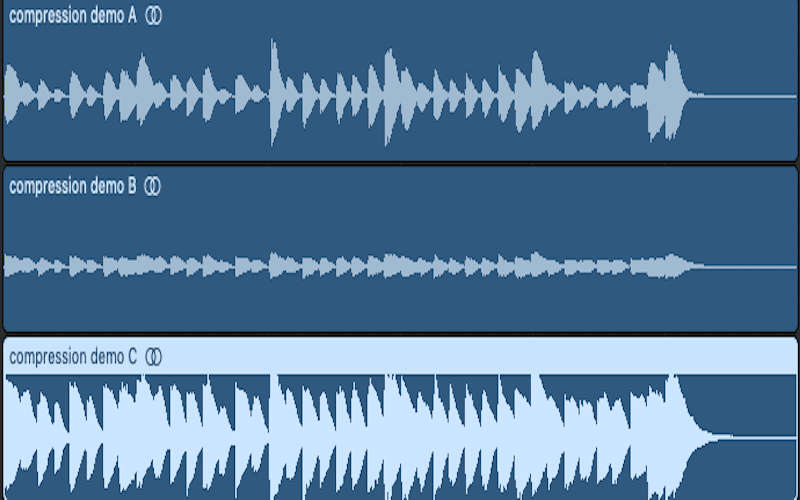
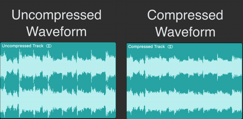
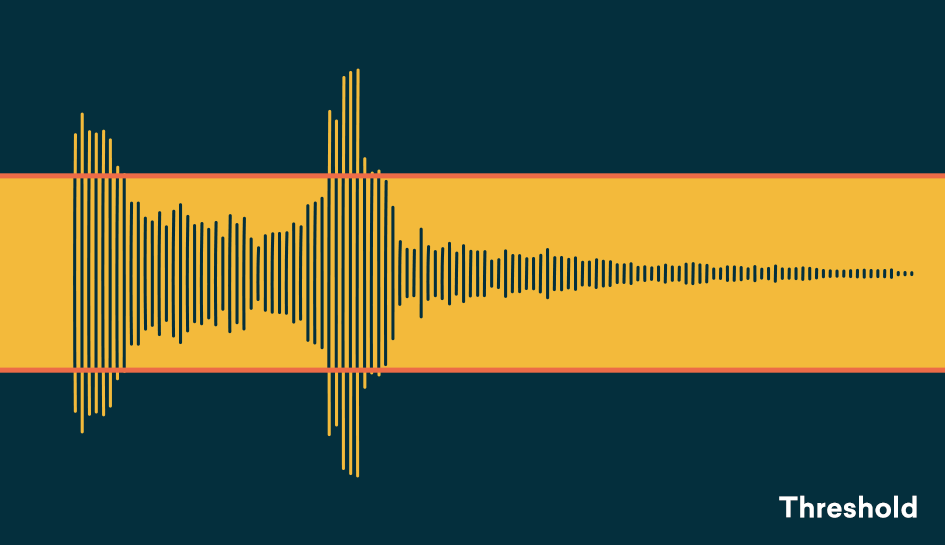
Compression in music is the process of reducing the dynamic range of a signal. Dynamic range is the difference between the loudest and quietest parts of an audio signal.

audio compression

You must reduce the dynamic range of most audio signals to sound natural to a recording.

For example: imagine a whisper and a scream on the same audio track. If they had the same volume difference as they do in real life, it would be very annoying!

Compressors fix all of this by attenuating the loudest parts of the signal and boosting what is output so that the quieter parts are more noticeable.

Imagine a whisper and a scream on the same audio track. If they had the same volume difference as they do in real life, it would be very annoying!
Using compression
Experienced engineers often talk about how one compressor is more “musical” than another.

It is an important concept. Its dynamics is one of the fundamental aspects for its sound to be unique.

When you use a compressor to change the dynamics, the sound engineer becomes part of the musical performance.

If your compressors work properly, they will positively contribute to performance and improve recordings.

Transients: understanding high energy moments.

To understand compression, you need to know what transients are.

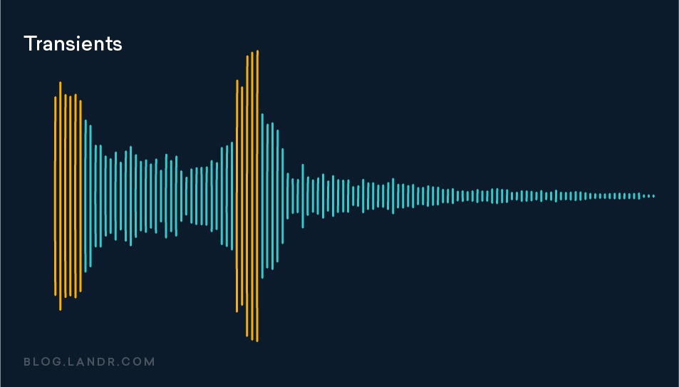
Transients are the first high-energy moments of a certain sound in its waveform. These explosions give our brain a lot of information about the quality of a sound.

Since transients are usually louder than the rest of the waveform, they are greatly influenced by compressors.

For example: think of a nice roaring trap. As soon as the trap enters, there is an initial peak in the waveform that narrows slowly. That initial energy spike is your transient.

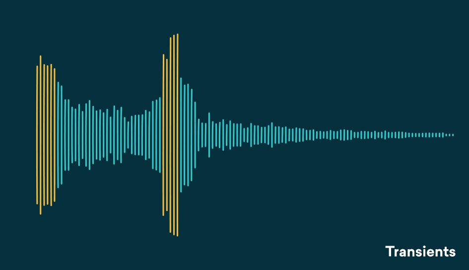
transient compresor

Compression helps you find the perfect balance for a track that has good dynamic range with a beautiful, full body.
A waveform with good dynamics will have a lot of transients when some sounds hit and then decay in the composition. Transients and their final decay are what make a waveform similar to a fish bone.

There is even an overly dynamic trail. If your song is transient without a body, its sound will not be of interest to your ear.

The reverse is also true, no dynamics can lead to lifeless, exhausting sound for the human ear and a waveform that looks like a big brick.

Compression helps you find the perfect balance for a track that has good dynamic range with a beautiful, full body.

Limiter

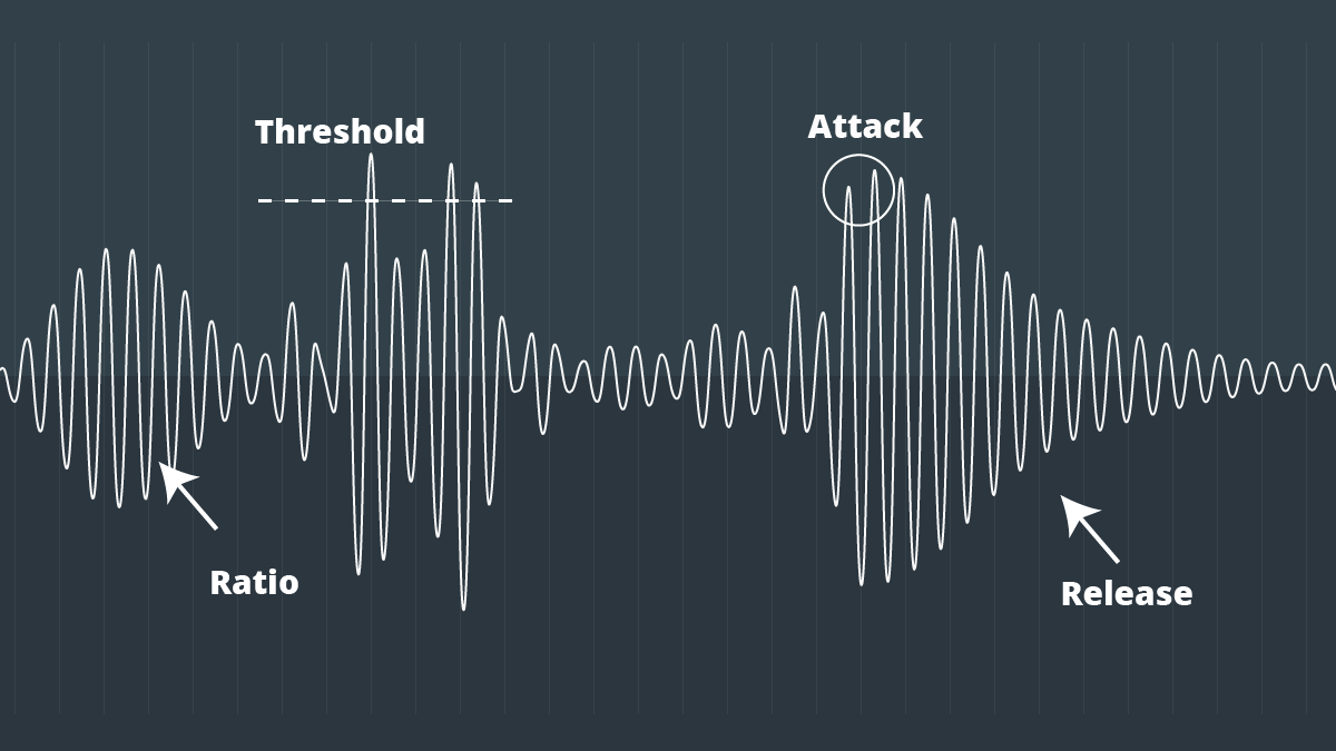
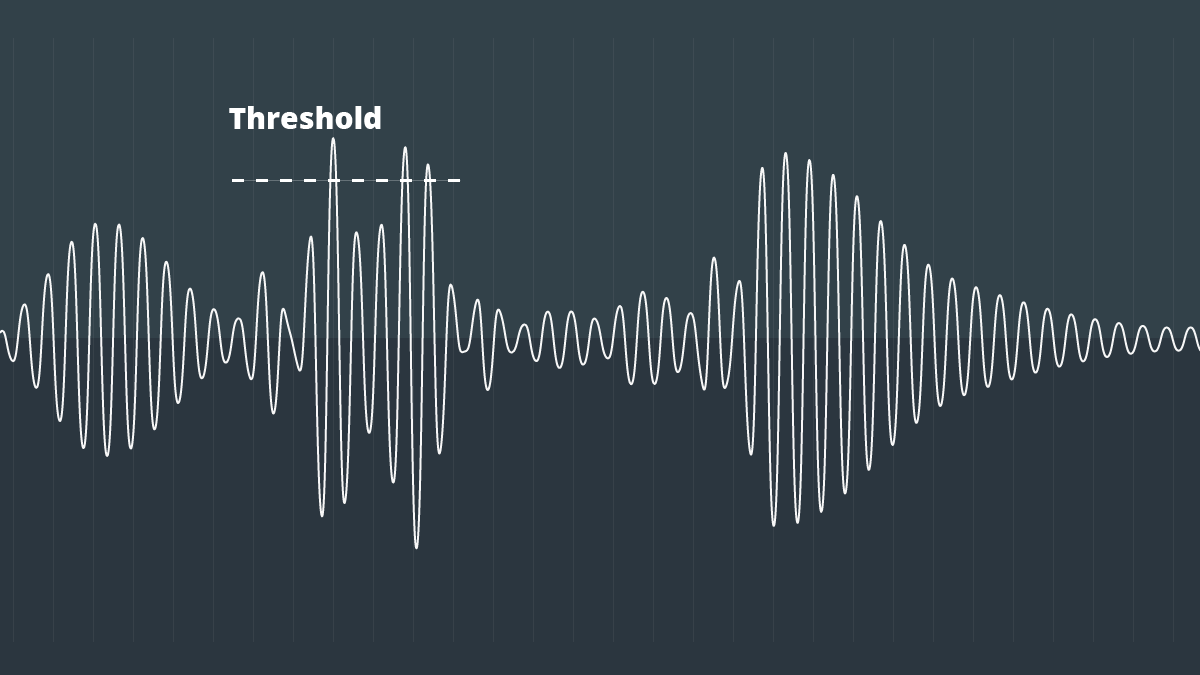
The threshold determines the signal level at which the compressor will start operating. The threshold is measured in dB, therefore any signal above the set threshold will be compressed.

When setting the threshold, decide what part of the signal you want to reduce.
With the threshold low, the compressor gain reduction is applied to a larger portion of the signal. Setting it higher affects only the most aggressive peaks and leaves the rest intact.

To determine what the perfect threshold is, think about what you’re trying to accomplish by compressing the audio and which parts of the signal are the most troublesome.

Are strong signal transients distracting you from the rest of your mix? Or maybe your final decadence is imperceptible in the mix?

A good rule of thumb for compression is “do no harm.”
Set the threshold to hear compressor operation on the part of the signal that needs to be addressed and not lowered.

Setting the perfect threshold will depend on your needs. Play the track and tweak it on the go to find the perfect amount.

Relationship

The ratio determines the amount of gain reduction applied by the compressor when the signal exceeds the threshold. It is called a relationship because it is expressed in comparison with the unaffected signal.

The higher the first number in the report, the greater the gain reduction factor.

For example, we can say that an uncompressed signal would have a 1: 1 ratio

What is the compressor and how does it work?

The compressor, together with the equalizer, is one of the most important and most used processors in professional audio, but its operation is not always so intuitive and knowing how to master the compression technique sometimes requires years of experience. In this new article we begin to explore this fundamental processor.

What is the compressor for?

First of all, let’s start to see what the compressor’s function is: to reduce the dynamic range of an audio track, that is, to decrease the distance in volume between the weakest signal and the strongest signal. Initially created to optimize recording on magnetic tape and to avoid saturation of the input stages, the compressor is still used today during recording and mixing. Reducing dynamic range also allows us to keep multiple tracks in the mix, such as a voice, for example, always at the same volume throughout the song so that they are not dominated by the other instruments in the most crowded sections, as well as to avoid Output saturation.

Compressor

Back to basics: what is the compressor and how does it work

The controls

Now let’s see in detail what the various compressor controls are and what they are for:
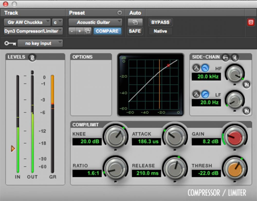
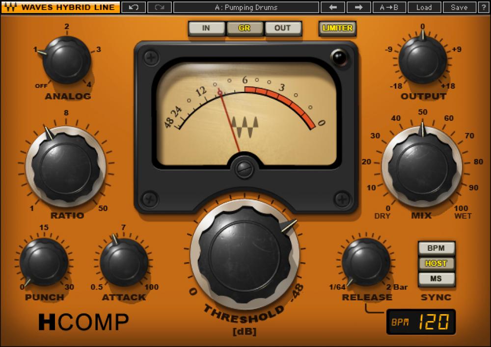
— Threshold: or threshold, expressed in dB, indicates the point beyond which the compressor begins to operate.
— Ratio: is the compression ratio and indicates how much the signal will compress when it exceeds the Threshold. For example, with a 2: 1 ratio, each signal that exceeds the threshold will be halved at the output, that is, every 2 dB at input 1 will be returned at the output.
— Make Up Gain: This is the output of the compressor and is used to recover the volume lost due to compression.
— Attack: expressed in milliseconds is the time it takes for the compressor to start once the signal has passed the threshold.
— Release: always expressed in milliseconds, it indicates the time it takes for the compressor to stop compression once the signal has returned below the threshold.
— Gain reduction meter: it is not a control but a visual indicator, led or pointer, which informs how much the signal is compressed, through a scale in dB.
— Bypass: shuts down the processor, making the signal pass through the machine without alteration.

With the advent of digital and accessories, we can find controls that not all hardware compressors have:
— Knee: indicates the type of curve at the point where the compressor begins to operate, which can be abrupt (Hard Knee), soft (Soft Knee) or various intermediate values.
— Automatic: sets the time control to which it refers (attack, release or both) automatically, depending on the input signal (program dependent).
— Sidechain eq or External Sidechain: Sidechain is the signal that drives the compression circuit, where in most cases it is the signal itself to compress, but sometimes it can be a version of the input signal with different equalization, for example without low frequencies, so that they don’t start the compressor too soon. Or it can be an external signal, such as the one used on the radio where the speaker’s voice signal drives a compressor on the background music signal, so it automatically turns off when it starts to speak (Ducking), or Classic Speaker Use to activate the compressor on various instruments in the mix or the Master Buss.
— Mix: used to mix the compressed signal with the original signal. This way, you can use Parallel Compression directly on the compressor, without having to use two mixer tracks (one for the dry signal and one for the compressed signal).
Back to basics: what is the compressor and how does it work

Compressor

Compressor or limiter?

What is the difference between a compressor and a limiter?

Essentially, the compression ratio: over 10 dB ratio, the processor is considered a limiter. A separate case is the Brickwall Limiter, a compressor with immediate attack and a compression ratio of infinity to 1, so that no signal can exceed the Threshold. It is mainly used on the master buses so as not to exceed 0dBFS on the output and then send the converters to clips.

Usage examples

As we already said, the compressor is used to keep the volume excursion under control. One track in the mix: in this case, using a fairly fast attack, slow release and not too aggressive ratio, allows us to compress the signal constantly and transparently, that is, without making your intervention feel excessively.
The compressor can also serve to emphasize the attack of a percussion instrument: in one case, for example, by setting a medium slow attack.