Why upsampling? Part 2


Free Download Mp4Gain
picture

Why upsampling? Part 2
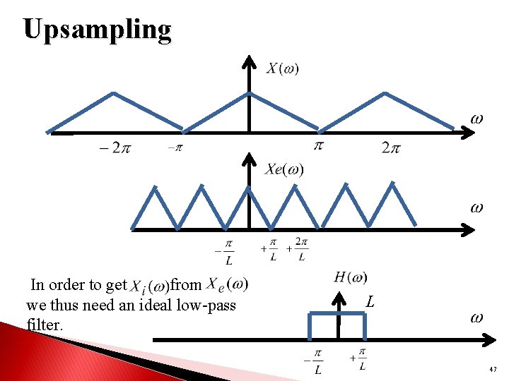
Upsampling

For every doubling of the sampling frequency, the spectral density of the noise is reduced by half and the signal-to-noise ratio increases by 3 dB. Since the resolution limit for the pressure level is approximately 1 dB, these decibels are unlikely to have a noticeable effect on sound perception in the high-frequency region. Based on these numbers, it is absolutely impossible to draw tentative conclusions about the change in sound quality.

In order to relate the spectrum of quantization errors, sampling frequency and sound quality, in this article it is proposed to use a tonal signal as a music model, as is usual to evaluate the quality of sound paths. This approach relies heavily on materials published in the “Sound Engineer” magazine.

The results can be summarized as follows. Unlike analog audio, digital audio is the product of amplitude modulation. This is manifested in a rigid functional dependence of the quantization error spectrum of the frequency multiplicity factor of the audio signal F and the sampling frequency fs, represented as the ratio of prime numbers y and x (k = fs / F = y / x). The frequency spectrum of quantization errors is always discrete and is determined solely by the multiplicity factor; the components of this spectrum are also determined solely by the amplitude of the audio signal, expressed in quanta. This means that the mechanism for shaping the quantization error spectrum does not depend on the number of bits used. With an increase in the quantization bit depth, the spectrum does not change in shape and composition, but only changes in level by 6 dB with each additional digit. (There are situations where a change in bit depth leads to a change in spectrum, – Ed.) The auditory perception of the quantization error spectrum is largely determined by the frequency response of hearing, which, in turn, it depends largely on the sound pressure level.

The frequencies of digital sound are divided into multiples when x = 1 and submultiples when x> 1. At multiple frequencies, the spectrum of quantization errors is harmonic and the main pitch is the frequency of the audio signal. If y is an even number, then the spectrum contains only odd harmonics. If y is an odd number, then the odd and even harmonics of the audio signal are present in the spectrum.

At multiple sub-frequencies in the quantization error spectrum, the components appear below the frequency of the audio signal, down to zero, and the lower limit of the spectrum Fn (x) is determined by the formula x – Fn (x) = F / X. In this case, the frequency Fn (x) becomes the fundamental pitch of the sound for quantization errors, and all other components, including the frequency of the sound signal, are converted to its harmonics. If the number is even at the submultiple frequency yskr, then the spectrum contains only odd harmonics of the frequency Fn (x). If yskr is an odd number, then the spectrum contains odd and even harmonics of this frequency. Low-frequency components in the quantization error spectrum lead to the appearance of harmonics in the form of pitch or consonance. They are especially noticeable at high frequencies in the audio signal when there is no frequency masking effect.

To clarify, we will give an example of a quantization error spectrum at an audio signal level of minus 30 dB with 8-bit quantization. Let fs = 48 kHz and F = 12800 Hz, then the multiplicity factor k skr = y / x = 48000/12800 = 15/4 and therefore the lower cutoff frequency Fn (x) = F / x = 3200 Hz, and the spectrum consists of odd and even harmonics of this frequency.

1.jpg

Figure 1. Quantization error spectra at submultiple frequency deviation

When the frequency of an audio signal deviates from a submultiple value by a small amount, sidebands appear around all harmonics of the spectrum, including zero (Fig. 1a), the number of spectrum components increases dramatically, and the limit bottom of the spectrum decreases, since the current value of x increases a lot.

Suppose, for example, that the frequency increment of the audio signal is 1 Hz, then the value of the multiplicity factor k = y / x = 48000/12801 = 16000/4267 and the lower limit frequency of the deviation spectrum becomes Fno = 12801/4267 = 3 Hz, and the interval between the components of the spectrum decreases to 6 Hz (Fig. 1b).


Free Download Mp4Gain
picture


Mp4Gain Main Window
picture


Mp4Gain Features
picture


Free Download Mp4Gain
picture

Why upsampling?

Why upsampling?

Upsampling

When it comes to improving digital sound quality, experts in this field agree on only one thing: with an increase in sample rate, sound quality improves dramatically.

Why upsampling?
When it comes to improving digital sound quality, experts in this field agree on only one thing: As the sample rate increases, the sound quality improves dramatically. Also, under the word “improvement”, everyone already understands something for himself. All the variety of opinions on this topic boils down to the following: the sound becomes clearer, softer, more natural, the low frequencies are perceived more clearly.

However, these nuances are only noticed by listeners trained with a good ear for music on specially selected sound material and using technically advanced equipment.

There are many hypotheses that explain why sound quality is improved by higher sampling. Many technicians are inclined to believe that this relationship is due to distortions that arise from filtering and interpolation during audio signal reconstruction.

On a modern technical level, high-quality interpolators may be practically impossible to implement, therefore, instead of improving them, manufacturers simply increase the sample rate. Maybe it’s not about them at all.

Another version, which many music lovers adhere to, is that at a low sampling frequency, for example 44100 Hz, digital sound is completely devoid of nuances of high sounds, the main frequencies of which are above 7 kHz. , and at lower frequencies there are very few harmonics for a high quality perception of music.

In fact, many musical instruments generate vibrations of up to 100 kHz. It is true that the fraction of energy that falls in the frequency band above 20 kHz is 0.01 to 2% for sounds of a harmonic nature and 0.02 to 68% for sounds created by a cymbal, triangle or striking the metal edge of a drum (hoop shot – editor’s note).

Even the frequency range of speech in hissing-hissing sounds extends up to 40 kHz. Supporters of this version are not ashamed that a person cannot perceive sounds with a frequency higher than 20 kHz. Ultrasound is assumed to be perceived bypassing the auditory system, for example through bone conduction.

Discussions that harmonics above 20 kHz make a significant contribution to sounding have culminated in the creation and widespread introduction of analog-to-digital converters using 96 kHz and 192 kHz sample rates; The sample rate is expected to increase to 384 kHz.

Based on modern knowledge of human perception of sound, it must be assumed that the relationship between digital sound quality and sampling frequency is due to the transformation of the quantization error spectrum in the audio frequency range.

In technical literature, this topic is considered only for a particular mathematical model, when music is represented by a signal with a uniform distribution in level and frequency. In this case, the quantization errors are converted to noise with a uniform spectral density from 0 Hz to the Nyquist frequency.

Relationship between sound quality and sample rate

Relationship between sound quality and sample rate

SAMPLE RATE

The conversion of an analog signal to digital consists of two steps: sampling in time and quantization in amplitude.

sample rate

Time sampling means that the signal is represented by a series of samples (samples) taken at regular intervals. For example, when we say that the sample rate is 44.1 kHz, this means that the signal is measured 44 100 times in one second.

The main problem in the first stage of converting an analog to digital signal (digitization) is the choice of the sampling frequency of the analog signal. The higher the frequency, the closer the digital signal is to the analog. However, in proportion to the increase in frequency, they increase:

The intensity of the digital data flow and the bandwidth of the interfaces are not unlimited, especially if several channels are recorded / played simultaneously;
The computational load on digital processors and their computing capabilities are also limited;
The amount of memory required to store the digital signal is increased.
Obviously, a compromise is needed. The choice of the sampling frequency affects the frequency range of the received digital sound and the maximum frequency of the analog signal, correctly represented in the digital one. It is believed that a person hears frequencies in the range of 20 to 20,000 Hz. According to the well-known Kotelnikov theorem, in order for an analog signal (continuous in time) to be accurately reconstructed from its samples, the sampling frequency must be at least twice the maximum audio frequency.

An audio frequency equal to half the sampling frequency is called the Nyquist frequency and is the maximum frequency that a given digital system can store and reproduce correctly. Therefore, if the actual analog signal that we are going to convert to digital format contains frequency components from 0 to 20 kHz, then the sampling frequency of that signal must be at least 40 kHz. The most common sample rates today are 44.1 kHz (CD) and 48 kHz (DAT).

The sample rate: looking for the best sound

When it comes to digital music and sound effects, the sample rate plays an important role. This applies to both CDs and file formats like MP3 and network players. The values ​​specified for the height or frequency of the removal rate differ significantly from each other. An important reference value is 44.1 kHz. We explain why this is so.

Sample rate

What is sampling frequency about

For a guitar voice or riff to be stored on a CD or hard drive, the sound must be digitized. To do this, samples of the analog signal are taken at constant time intervals (discrete time). These are used to convert the recorded information into a code.

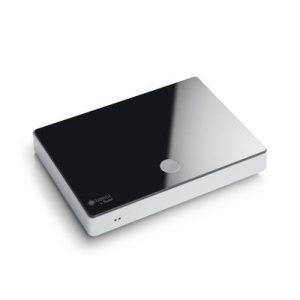
Raumfeld connector
Raumfeld connector

If the signal is digital, such as MP3, it can also be converted back to an analog signal, such as fluctuating current intensity, to make the membrane of a speaker sound. The frequency of these samples or samples is indicated by the sampling frequency. In general, the more samples there are, the more detailed the sound can be digitally reproduced.

A CD accepts signals that have been digitized with a sampling frequency of 44,100 Hz or 44.1 kHz. That corresponds to 44,100 samples per second. Of course, this frequency was not determined by chance. Such a resolution takes into account the maximum audible audio frequency of about 20 kHz and an important rule of data processing: the Nyquist-Shannon theorem. From this it can be deduced that the sampling frequency must be at least twice as high as the highest frequency of the signal to be digitized. So if the highest tones we can hear vibrate at 20 kHz, according to this theorem, the sample rate must be at least 40 kHz in order to digitize and decode all the tones correctly. Otherwise, the digitized signal can only be incorrectly converted to analog.

44.1 kHz is not the end of the story

The sampling frequency development did not stop at 44.1 kHz. Modern data carriers and transmission methods now make it possible to process significantly larger amounts of data. Lossless formats like FLAC or high resolution multi-channel standards exceed this value many times over.

Dolby TrueHD, for example, supports very high sample rates. Thus, significantly finer digitized signals can be processed. Additionally, audio masters can use better reconstruction and anti-aliasing filters.

Sample rate isn’t the only measure – bit depth

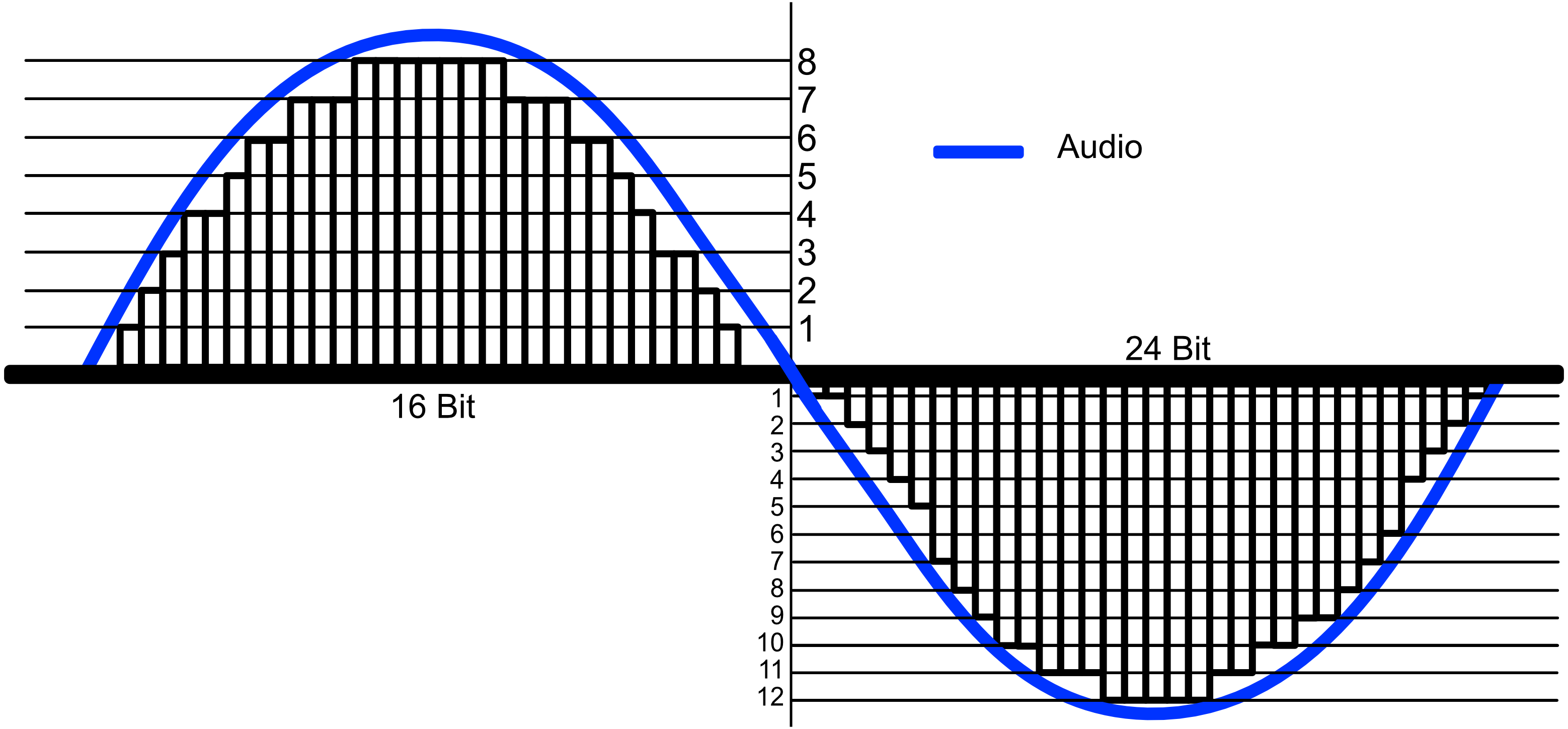
While the sample rate describes the frequency of the samples, the bit depth indicates how many bits are used per sample. In other words, the bit depth tells you how accurate or how high the resolution is for each individual sample. The amplitude or dynamic range of the analog signal at the time of the sample is determined. So the area between the weakest and strongest sound pressure level. On a CD, each sample is 16-bit deep, although this value is also exceeded by modern digital standards. Dolby TrueHD reaches 24 bits.

The Raumfeld connector brings out what is digitally possible
The raumfeld connector supports a sampling rate of 192 kHz.

▶ Hardly anyone makes bits sound as good as the Raumfeld plug. Because it plays high-resolution formats up to 96 kHz and 24-bit. An integrated high-end converter from Cirrus Logic converts digital data into analog. The Raumfeld connector has a powerful WLAN module for wireless data transmission. Thanks to Google Cast, multi-room speakers can also be conveniently controlled via the connector. If you connect the network player to a conventional system via Cinch or Toslink, it will be integrated into the local network.

Conclusion: sample rate as a bargaining chip for digital sound formats
The sampling rate indicates how often signals are sampled from an analog signal for digitization.
The Nyquist-Shannon theorem states that for the digitization to be true to the original, the sample rate must be at least twice the highest analog frequency.
CDs support sample rates up to 44.1 kHz. Modern formats, on the other hand, can reproduce 96 kHz and more.
Bit depth indicates how individual samples are resolved and influences the digitized dynamic range.
While CD samples have a 16-bit resolution, Dolby TrueHD, for example, reaches 24-bit.

Sample rate (Hz and kHz), resolution (bits), and bit rate (kBit / s) for music and audio

Because it always leads to misunderstandings, today there is a short explanation of the most important key figures for music and audio files. These basically apply to all uncompressed formats (WAV and AIFF). I’ll also go into the bitrate of compressed formats like MP3, WMV, and OGG below.

Sample Rates

Basic knowledge: An audio file stores a number at very short intervals that represents the level of the audio signal. During playback, the contour is calculated from this sequence of numbers.

Audio Sample Rate

An audio file can have multiple channels. Mono (one channel), stereo (2 channels), and 5.1 and 7.1 (Surround) are common. Each channel provides the information from one of the speakers and is a separate audio signal. That means we can split a stereo file and save it into two mono files.

The sample rate (Hertz) indicates how often the audio level is recorded and saved in one second. A specification of 44,100 Hz (44.1 kHz) means that 44,100 values ​​are stored for one second of music. Typical sample rates are 44.1 kHz (music CD), 48.0 kHz (film), and 96 kHz (recording studio).

The resolution (bit) indicates how much memory is used for that sample value. For example, 16 bits (2 to the power of 16) allow a scale of 65,536 values ​​for each individual sample value. If we have a lot of memory for a value, we can process the signal more precisely. Typical settings are 16-bit (music CD) or 24-bit or 32-bit in the studio.

Bit rate (kBit / s) is often confused with resolution. Represents the “bandwidth” of the audio file, that is, the amount of data that is processed in one second. For uncompressed formats like WAV and AIFF, you can easily calculate the bit rate by multiplying the above three values:

Bit rate = channels x sample rate x resolution

Example:

A WAV file in CD quality has the following bit rate:
2 channels x 16 bits x 44.1 kHz = 1411.2 kBit / s

The bit rate for compressed formats (MP3, OGG, WMV, AAC, etc.)
Unfortunately, this formula does not work with MP3 and other compressed formats because the signal is packaged to save space. The encoder reduces the bandwidth of the data to a desired bit rate and tries to obtain the best possible quality within this frame. The bit rate can be constant (CBR mode) or variable (VBR mode). A variable bit rate often makes sense if the audio signal is highly varied (for example, a movie or radio playback).

Sample Rate

Sample Rate

The seconds are defined by taking as a time sample the period of oscillation of the light waves emitted by a cesium 133 atom in a particular atomic transition.

As we have already observed in the dedicated paragraph, sound is generated by small variations in atmospheric pressure that propagate in space and time and until the end of the 40s of the last century it could only be transduced by the human auditory system or by the microphone devices used. for the transmission of signals by radio but it cannot be stored in any type of support dedicated to mass cultural diffusion. In fact, there were already several technologies dedicated to the memorization of sound waves but they were either of poor quality and diffusion such as phonographs and gramophones or were used only experimentally or were dedicated to communications between military devices.

The only vehicle to transmit sound events for musical purposes was still the score that had to be interpreted by a human interpreter and, if someone wanted to listen to a certain piece of music, they had to go to a theater or concert hall that had it on the bill. We emphasize that the performance (as well as the listening) was unique and non-repeatable and the only memory capable of preserving the sounds was the human. All this until 1948, when in the United States Columbia patented the first 33 rpm vinyl record in the 25 and 30 cm formats and where the waveform (as previously happened with 78 rpm records) was printed in micro-grooves that were They developed in a spiral along the surface of the disk and were read by one of the giradichi heads.

The following year (1949) another type of media dedicated to the preservation and reproduction of sound was also introduced on the market: the first magnetic tape recorders wound on reels and later in 1964 Philips commercialized the four-track cassette in Europe. The era of massive musical (and cultural) enjoyment has begun, which after hundreds of years has profoundly and definitely changed our relationship with the world of sounds.

All the means and systems for storing sound waves that we have just exposed (in addition to others that I have not considered appropriate to mention here) belong to the world of analog audio since the information or rather the representation of the sound wave is produced in a continuous and analogous to the original changes in atmospheric pressure. This is because analog recording devices (transducers or microphones) transform changes in atmospheric pressure into changes in the voltage of an electrical signal, which can be stored on mechanical (vinyl records) or electromagnetic (magnetic tapes) media. to be eventually reproduced one or more times at later times. This, in addition to being a transcendental technological revolution, has also greatly influenced the diffusion of music in society, the role of music within it and the development of languages ​​closely linked to the sound or musical arts.

In 1971 a new revolution began which, however, this time is strictly technical (from the cultural and social point of view it only amplifies and accelerates the process of global dissemination of information already underway): the birth of digital audio. In fact, in that year the research laboratories of NHK (Japanese public television radio) created the first digital audio recorder that, using the PCM (Pulse Code Modulation) technique patented by the British A.

Sampled signal

We have said that sampling a signal means measuring its amplitude (y) in each sampling period, obtaining a discrete signal in time and continuous in amplitude:

Sample rate

At this point, however, we are faced with a question: how often to sample the signal? Theoretically we can say that the shorter the sampling period, the less information will be lost between one sample and the next, obtaining a digital signal more similar to the original up to the ideal limit (infinitely small period) in which the analog signal and the sampled.

Sample rate

In practice, however, there are technological limits in the construction of ADC converters that do not allow us to achieve such short periods. Therefore, we must start from the assumption that the samples must be taken with a speed dependent on the variation of the signal and this speed depends on the harmonic component of higher frequency that will determine the sampling period.

Sample rate, a clear explanation about what the sample rate is

Let’s proceed in order and start from the sampling frequency, defined as the number of times per second in which our AD converter will measure the electrical signal placed at its input: it is measured in Herz (Hz).

Obviously, the greater the number of “photographs” that we take of our electrical signal in one second, the greater its fidelity to the “original” sound wave. At the same time, obviously, our converter will be obliged to spend a greater amount of “energy” (faster information processing speed, greater storage space, etc.) which therefore translates into a different quality of components and obviously at a higher cost.

La tasa de muestreo

Sampling rate

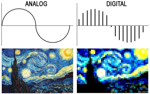
On the left an analog wave (a sine wave) in the time / amplitude domain and an image of Vincent Van Gogh’s “Starry Night” which, for our teaching purposes, we intend to be very high resolution. On the right, a quick reconstruction of the same sampled analog waveform and the same photograph reproduced with a much smaller number of pixels.

Well, if it were that simple, there wouldn’t be a bit of fun. Let’s go back to the diagram of the AD converter at the end of the previous article. Surely you have noticed that the first block through which our signal passes is the so-called “Anti-aliasing filter”, nothing less than a low pass filter.

Coooooooooooosaaaaaaaaaaaaaaaaaa !? Do we want to faithfully reproduce our signal in the digital domain and the first thing we do is pass it through a filter to change its frequency component (remove all components above a certain frequency)?

Yes my dear … you need to share a minimum (but I swear, a minimum) of signal theory to tell you a bit about the “Nyquist-Shannon Sampling Theorem” (for the “fetishists” – no offense, for course …. I am also part of it: of the mathematical treatment, take a look at the related Wikipedia page where you can find a good perspective), based on which, to sample an analog signal without loss of information (that is, to be able to re-enter it – then convert it DA – into the analog domain without “noticeable” differences compared to the original signal) it is necessary that the number of samples taken per second (the sampling frequency) is at least twice the maximum present frequency into the signal to be sampled, Therefore, it is worth introducing frequencies in the digital signal that do not exist in the original analog signal (the calls, and hence the filter name, alias frequencies).
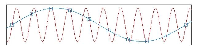
The aliasing phenomenon occurs because we do not have enough samples to describe the trend of the higher frequencies, which are therefore translated into the digital signal as lower frequencies, although nonexistent in the original signal. See this beautiful image always taken from the omniscient Wikipedia. In red the sinusoid sampled at intervals not sufficient to reconstruct it, and in blue the frequency alias (lower) that originates from the points we have taken.

La tasa de muestreo

Sampling rate

As we already know, the human ear is sensitive, at most (at an early age and in good hearing health), to frequencies around 20 KHz; In theory, our anti-aliasing filter should be set at 40,000 Hz and that should be our sample rate, but since it is practically impossible to build a filter with such a steep slope in analog, we opted for a filter with less steep slope and so both leaves the signal to sample frequencies slightly higher than 20,000 Hz (which we don’t hear, but there are), sampling at a slightly higher frequency. Therefore, the minimum sample rate used is equal to 44,100 samples per second.

Obviously, technological development and, nevertheless, the opinion and experience of many professionals (which I personally share very modestly) have in any case led to the awareness that, having set the minimum limit of 44,100 Hz (we will see later, it is the sampling frequency of the files that make up an audio CD), sampling at higher frequencies certainly leads to better results both from the point of view of signal manipulation (passing through a plug-in, the sum of two or more signals within a DAW, etc.) and from a listening point of view.

Later we will return to the topic, we will develop it further and we will begin to understand the logic with which the converter assigns a value in “machine language” to the different samples taken during the sampling phase.