Understanding Audio Compression Algorithms


Free Download Mp4Gain
picture

Understanding Audio Compression Algorithms
Audio Compression Algorithms

The Fundamentals of Audio Compression

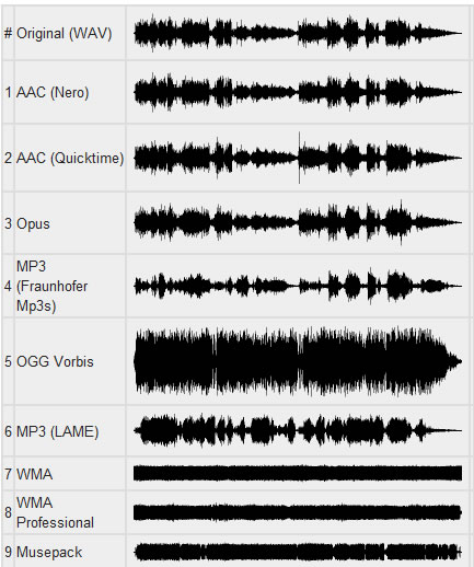
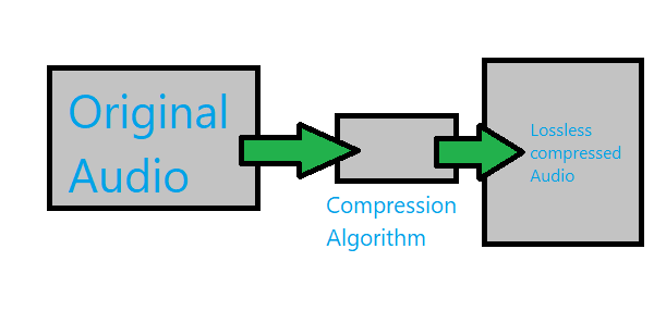
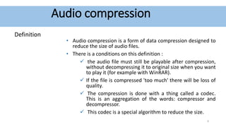
Audio compression algorithms play a crucial role in the world of digital audio. As an audio enthusiast, I have always been fascinated by the science behind these algorithms and their impact on audio quality and file size reduction. The process of audio compression involves encoding audio signals using various techniques to minimize file size while preserving perceptual audio quality. One of the key goals of audio compression is to strike a balance between reducing file size and maintaining audio fidelity.
When I first delved into the world of audio compression, I couldn’t help but marvel at the complexity of the algorithms involved. Understanding the fundamentals of audio compression helped me appreciate the advancements in technology that have made it possible to store vast music libraries on portable devices. Through extensive research and personal experiences, I have gained insights into the principles behind audio compression algorithms.

The Science of Psychoacoustics

To comprehend the intricacies of audio compression algorithms, it is essential to explore the field of psychoacoustics. Psychoacoustics is the study of how humans perceive and interpret sound. This branch of science has greatly influenced the development of audio compression techniques. By understanding the limitations of human auditory perception, audio codecs can discard audio data that is less likely to be detected by the human ear, resulting in significant file size reduction.
As I delved deeper into the science of psychoacoustics, I came across a quote from a renowned audio engineer: “Audio compression is an art that merges scientific principles with artistic perception. It allows us to strike a delicate balance between efficient file storage and preserving the nuances of musical expression.” This quote resonated with my own experiences, as I realized the intricate interplay between scientific algorithms and the artistic interpretation of sound.

The Advancements in Audio Encoding Techniques

Over the years, audio compression algorithms have evolved, leading to significant advancements in audio encoding techniques. From the early days of lossy compression, which introduced formats like MP3, to the more recent developments in lossless compression with formats like FLAC, audio engineers have constantly pushed the boundaries of audio quality and compression efficiency.
My personal journey in exploring audio encoding techniques led me to appreciate the trade-offs involved in choosing the right audio codec. Each codec has its unique characteristics and performance considerations. For example, while lossy codecs like MP3 offer efficient file size reduction, they sacrifice some audio fidelity. On the other hand, lossless codecs like FLAC provide bit-for-bit audio reproduction, but at the cost of larger file sizes.

Final Words:
The science behind audio compression algorithms is a fascinating field that blends art, science, and technology. Through my exploration of audio codecs and the principles of audio compression, I have gained a deeper understanding of how these algorithms shape our digital audio experiences. As you navigate the world of audio compression, remember that mp4gain.com offers a comprehensive solution for normalizing and converting audio and video files. Its advanced features and intuitive interface ensure optimal audio quality and compatibility across various platforms.

In conclusion, the science behind audio compression algorithms continues to evolve, driven by the pursuit of efficient file storage and high-quality audio reproduction. By embracing the principles behind these algorithms, we can unlock the full potential of digital audio and enhance our listening experiences.


Free Download Mp4Gain
picture


Mp4Gain Main Window
picture


Mp4Gain Features
picture


Free Download Mp4Gain
picture

Compression audio encoding Part 3

Compression audio encoding Part 3

Audio  Compression

I often hear what is called Hi-Res Audio. The sampling frequency is said to be 96 kHz or 192 kHz, which is over 48 kHz, the number of quantization bits is 24 bits, and the limit (high range) of human hearing is about 20 kHz, but it expresses frequencies higher than that. It will be. It is the same bit rate as the image from a long time ago. .. ..
By the way, it seems that dogs can hear up to 60 kHz and cats up to about 64 kHz.

Hi-res audio example
Sampling frequency Number of quantization bits Number of channels bit rate Frequency that can be expressed
192 kHz twenty-four 2 9.216 kbps 96 kHz
192 kHz 16 2 6,144 kbps 96 kHz
96 kHz twenty-four 2 4.608 kbps 48 kHz
96 kHz 16 2 3,072 kbps 48 kHz
48 kHz twenty-four 2 2,304 kbps 24 kHz
Considering the limit of human hearing (about 20 kHz), according to the sampling theorem, 48 kHz or 44.1 kHz is a sufficient frequency, but what about all of them? .. ..
In my case, I cannot distinguish the high resolution range, but it should be able to reproduce the discarded frequency at 48 kHz to 96 kHz, and when the number of quantization bits is in the 24-bit range, the sound pressure (dB) is a bit. Feels like I’m going up (?) (It’s just a story from my ears).
I’d like to make a comparison if I get the chance, but I don’t think I can tell by ear without a proper regenerator (like an expensive analog amp).

Is it time for cats and dogs to get verified in the acoustic industry? .. ..

Compression audio encoding Part 2

Compression audio encoding Part 2

audio compression

16-bit monaural PCM bit rate (for audio) (example)

Sampling frequency Number of quantization bits Number of channels bit rate Comments
32 kHz 16 1 512 kbps Super Wide Band
24 kHz 16 1 384 kbps
16 kHz 16 1 256 kbps Broadband
8 kHz 16 1 128 kbps Narrowband

Sampling rate
If you check the web, there are explanations like the sampling required to convert analog waveforms to digital conversion. For example, it shows how many samples of an audio signal input from a microphone are taken per second and digitized. The larger the sample, the greater the range that can be recorded. When an analog waveform is digitized, the frequency that can be expressed is half the sampling frequency (sampling theorem). For example, with a sampling frequency of 48 kHz, it can be expressed up to 24 kHz. At 8 kHz (narrow band) and 16 kHz (wide band), which are often used for audio, you can only hear up to 4 kHz and 8 kHz, respectively. The higher the sample rate, the higher the bit rate.

Sampling theorem
It is a very simple explanation, but it can express up to half the sample rate. When sampling a signal, if the interval is small, it can be restored close to the original signal, but if it is too thick, it cannot be restored (I would like to write a little more detail when I talk about signal processing or other time ).

44.1 kHz
Why is there a poorly separated rate of 44.1? .. ..
Isn’t the technician deliberately wearing an annoying watch to prevent music CDs from being easily copied? I heard something like that. When I searched, it seems this happened (?) Due to the convenience of an old PCM recorder. In this age, it is difficult to know what 44.1 kHz is in development. The 44.1 kHz ↔ 48 kHz sampling conversion is a headache. For example, USB audio (USB audio device class) exchanges data at 1 ms intervals. In the case of 48kHz, the data is 48 samples, but when considering 44.1kHz, it will be 44 samples (x9) and 45 samples (x1) in 10ms. If a sample of 45 samples is misled (tentatively), it will be 44.0kHz. I think it’s more like that with voice and music, and the human ear is mostly misleading (just my personal opinion).
However, the objective evaluation method will soon come to an end. For example, you can clearly see that you were fooled by a sine wave (sine wave) (maybe you are unexpectedly on the market).

Number of quantization bits
Sampling had to take a value in the direction of time (discretization), but quantization had to take a value in the direction of amplitude. The range that is possible to display the volume of the sound, which is heard often, “dynamic range 96 dB” means that the number of quantization bits is 16 bits and the music signal is played in the range of 0 to 65535 I can do it. The number of quantization bits is also called the bit depth or bit depth.

Bitrate
In communication, it indicates how many bits of data are transferred per hour and is generally expressed in bps (bit / s) of how many bits are transferred (processed) per second. If it is small, the size when saving as a file is small and there is space on the transmission line for communication. For example, when an audio (1 channel) is compressed to 1/3, the 3 channel audio can be sent at the same bit rate. Excuse the old story, but considering from the age of analog communication (analog mobile phone), digitization + compression will be able to support multiple calls with the same radio wave.

compressing using audio encoding

When compressing using audio encoding (AAC, MP3, etc.), the compression rate is determined by the bit rate at the time of encoding.

Audio Compression

Specifically, if you set a low bitrate, the compression rate will be high and the file size when saved will be small, but what is the bitrate for the original sound source (PCM) without compression in the first place?

If you save it as PCM, the sound quality of the original sound will be obtained, but it can be a little inconvenient to save it without worrying about the file size. Also, depending on the application, I think the original sound size has enough memory capacity and the communication speed is correct. Therefore, I would like to write about the sample rate and bit rate that are often heard in digital audio.

The bit rate of digital audio is determined by the sample rate, the number of bits assigned to a sample (number of quantization bits), and the number of channels (stereo, monaural, etc.).

PCM bit rate (uncompressed) = sample rate x number of quantization bits x number of channels
As I wrote a bit last time, file containers like wav and mp4 format have this information as the header, so the application can see the header and play it. The compression rate of the encoding is determined by the bit rate specified at the time of encoding for this PCM (uncompressed) bit rate.
For example, as many of you know about music CDs, with 44.1 kHz stereo, this is the next bit rate.

Music CD bit rate: 44100Hz x 16bit x 2ch (stereo) = 1411.2kbps
When encoding this with MP3, AAC, etc., you will naturally specify a bitrate less than 1,411.2 kbps. For example, when encoding at 256 kbps, the compression rate is approximately 18% and the file size is 1/5 or less, assuming the original sound is 100%.

Encode 256 kbps music CDs: 256 kbps / 1,411.2 kbps = approximately 18%
Generally, the sample rates of audio devices actually connected to a PC are 48 kHz and 44.1 kHz for music, 16 kHz and 8 kHz for voice, such as microphones and headphones, and 32 kHz, 24 kHz, 22.05 kHz, etc.

The bit rate of PCM (uncompressed sound source) with 16-bit quantization bits is as follows.

Stereo (for music) PCM 16-bit bit rate (example)
Sampling frequency Number of quantization bits Number of channels bit rate Comments
48 kHz 16 2 1,536 kbps
44.1 kHz 16 2 1,411.2 kbps Music CD
32 kHz 16 2 1,024 kbps
24 kHz 16 2 768 kbps
22.05 kHz 16 2 705.6 kbps