Sample rate and bit depth


Free Download Mp4Gain
picture

The comparison with the digital or film camera is not completely random: the sampling frequency of the audio signals, that is, the frequency of the samples per unit of time (usually given per second), is comparable to the frame rate per second from a film camera. The number of pixels in each individual image could be equated with the bit depth: HD movies “look better” than Super 8 movies. The higher the number of pixels on the sensor and the more often a photo is taken, more precisely, the “light to be recorded”, the landscape, can be digitally reproduced.

Bit Depth

Bit depth

Fortunately for us, a certain Harry Nyquist inspired a certain Claude Shannon long ago to support him with a theorem (a theoretical statement or theorem) that stated that an audio signal at twice the frequency must be sampled uniformly to match. with the original signal. to be able to rebuild sufficiently. Limiting the bandwidth of audible frequencies practically frees us from our hearing, which is basically only capable of consciously perceiving frequencies between a maximum of 20 Hz and 20,000 Hz.

Sample rate

The expense of completely and exactly reconstructing the analog output signal is theoretically infinite, since digital signals are discontinuous by nature in any case, while analog signals are always continuous. Unfortunately, it is inevitable that digital information is only suitable for rough storage of analog signals. The starting signal is “rough”, good word, right? Nyquist’s theorem also applies to digital cameras: they also deal with frequencies, that is, those of light.

digital audio

For signals up to 20 kHz more or less relevant to humans, a sampling frequency of 40 kHz is sufficient according to the aforementioned theorem. The 44.1 kHz sample rate common for CD quality comes from the 1970s or Sony’s “pulse code modulation (PCM) process for storing digital signals on video tapes. Later, Sony developed the Red Book standard for audio CDs with Philips.

The frequency, which is slightly wider by an additional 4000 Hz than twice that audible to humans, has its origin in the simplest possible filters, which are intended to remove so-called aliasing effects from the audible range of the reconstructed analog signal. during digitization: the wider this “corridor”, the simpler the filter technology.

PCM pulse code modulation method

Exactly 44.1 kHz got out of this, because sample rate converters can be more easily designed (used for studio technology or data carrier transfer) if the sample rate is an integer multiple of the output frequency. The output frequency here was the 60 Hz network frequency used for video digitization with 525 lines to digitize the TV signal. Changing 60 Hz would have been very laborious, it stuck. It is not a coincidence that multiplying 525 by an integer factor results in a frequency greater than 44,000 Hz, which we want to achieve to keep filters for anti-aliasing simple: the next largest integer that is divisible by 525 is 44,100. The multiplication factor is 84, as a whole number is desired, which should not interest us otherwise.


Free Download Mp4Gain
picture


Mp4Gain Main Window
picture


Mp4Gain Features
picture


Free Download Mp4Gain
picture

Multimedia formats: Digital audio


Sound is a continuous signal. To be stored with computer systems
it must be sampled, thus obtaining a digital signal.
The parameters that characterize the sampling are basically three:

 The sample rate
 Bit depth
 The number of channels
these parameters influence both the space occupied and the quality of the audio file
digital obtained.

Digital Audio

Sampling rate

The sampling frequency is the measurement expressed in Hertz (Hz) of the number
of times per second in which an analog signal is measured and stored
in digital form.

Sampling rate
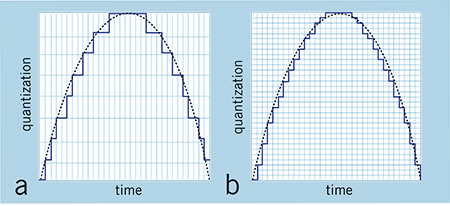
The higher the sampling rate, the more the sequence of the samples
digital will be close to that of the original analog waveform.
Low sampling rates limit the frequency range that is
can record, which in turn can generate a recording that
poorly reproduces the original sound.
Two sampling frequencies:
A. Low sampling rate,
which distorts the wave of the original sound
B. High sampling rate,
which perfectly reproduces the wave of
original sound
To reproduce a certain frequency, the sampling frequency
it must be at least double it (Nyquist theorem).
For example, audio CDs have a sampling rate of 44.100 Hz,
so they can reproduce frequencies up to 22.050 Hz, which are hardly found
beyond the limit of human perception of 20,000 Hz.
The following table shows the most common sampling rates for
digital audio.

Bit depth

The bit depth represents the number of bits used to store a
single digital sample.
When a sound wave is sampled, each sample is assigned
the amplitude value closest to the original wave amplitude. A depth
in high bits it provides as many amplitude values ​​as possible, which results in a
greater dynamic range (the difference in decibels between the maximum volume that the component can sustain without
distort the waves and the background noise it produces), lower and higher background noise
fidelity.
For example if you use 8 bits you have 256 possible values ​​(28
) that, being
relatively few, offer less sound quality than a
tape; if instead 16 bits per sample are used, 65536 values ​​are obtained
possible (216).
The most common examples are the audio CD, recorded in 16 bit, and the DVD, which
supports up to 24 bit depth.

Compression formats

Hand in hand with the advent of digitalization, multimedia applications have
they are increasingly widespread until they become commonplace. One of
multimedia features is certainly the use of digital audio
vowel and sound. The biggest obstacle associated with digitizing audio is
the large size of the files that are produced, which puts them at
sector operators (especially those linked to the internet) the problem of
reduce the space occupied by the data to obtain the double advantage of:
 save in terms of memory occupation;
 save in terms of transfer time on the network.

For this reason, speaking of digitizing the audio, it is necessary to speak
also of data compression techniques. The compression techniques of the
data, of whatever nature they are, are divided into:
 lossless: compress data through a lossless process
of information that takes advantage of redundancies in data encoding
 lossy: compress data through a lossy process
of information that takes advantage of redundancies in the use of data.

Lossless formats

Lossless compression formats are more suitable for archiving rather than
to reproduction, since most of them require complete
decompression before they can be played.
One of the most common lossless compression formats is FLAC (Free Lossless Audio Codec).

Lossy formats

Lossy compression formats use compression algorithms capable of
drastically reduce the amount of data required to store a sound,
guaranteeing however an acceptable and faithful reproduction of the original file uncompressed.