what should the sample rate be set Archives - Page 5 of 5

Understanding Sample Rate Part 2

Free Download Mp4Gain

Understanding Sample Rate Part 2

sample rate

When the number of samples is reduced in this way, the original smooth curve disappears and a choppy waveform is created.

Sample Rate

Well, when it’s actually played back, it’s not the reason the signal is so choppy, it’s that in post-processing by the computer, “From the position of this point, the original waveform would have looked like this.” it is possible to reproduce a certain curve, but…

However, it is easy to imagine that the smaller this point is, the more difficult it will be to reproduce the original correct waveform, right?

In other words, you can understand that the higher the sample rate, the higher the reproducibility of the original sound.

Let’s hear the difference in sound quality depending on the sample rate

Let’s see in this video how the sound quality actually changes when the sample rate is different.

In this video you can check the sound quality of each of the four stages, “8kHz, 16kHz, 32kHz, 48kHz”.

There is a clear difference, right?

At 8kHz, the treble is cut off so much that it doesn’t seem to be the same song, and the overall muffled sound makes it impossible to hear the drum hi-hat.

The higher the sample rate, the better?
As you can see in the video above, sample rate is an important part of sound quality.

At this point, it’s easy to think, “If you set the sample rate to 96kHz or 192kHz, you should get really good sound!”, but actually the change in sound is quite hard to understand after 44, 1kHz

So why is it difficult to understand the change in sound after 44.1 kHz?

The reason why the change in sound quality is difficult to understand above 44.1 kHz
First, the frequency band that humans can hear is determined to be “20 Hz to 20 kHz”.

And as the basis of audio, there is a rule that the sample rate “needs twice the frequency of the frequency band you want to reproduce”. (For more information, see “Nyquist Frequency”)

Simply put, if you want to play down to 20kHz, which is the human audible range, you need a sample rate of at least 40kHz.

Since the sound quality of the CD is 44.1 kHz, the CD can completely cover the limit of human hearing, 20 kHz.

In the video above, the sound source with a sampling rate of 8 kHz is actually 4 kHz or later, and the sound source with a sampling rate of 16 kHz is actually 8 kHz or later, and the high-pitched sound disappears.

daughter
That’s why I couldn’t hear the high-frequency hi-hat sound at first.

At this level, the difference is easy to understand because it is within the human audible range, but since the CD sound quality has already been reproduced beyond the human audible range of 20 kHz, the playable frequency becomes 48 kHz or 96kHz So in most cases, the general public either don’t have enough speakers or headphones to reproduce it, or they can’t hear frequencies above 20kHz in the first place.

However, there are some interesting research results that humans hear components above 20kHz, so you can’t say there’s no point in playing after 20kHz, but unless you’re listening in a very good environment. There’s no doubt that most people can’t tell the difference.

Reference: Effect of components above 20kHz on the perception of instrument sounds

Three reasons why a 44.1 kHz sample rate is enough

So far, you know that as the sample rate increases, the difference in sound quality becomes negligible.

So what value should be set for the project sampling rate?

It’s “44.1kHz”!

Let’s look at why 44.1 kHz is the recommended sample rate, along with three reasons why.

The higher the sample rate, the higher the CPU load.
This is the biggest disadvantage of increasing the sampling rate.

If you increase the sample rate of the project, the load on the CPU will increase and the computer will not work properly.

Therefore, the higher the sampling rate, the greater the amount of information, but it is not a good option to demand too much sound quality with the specifications of a general personal computer.

After all, the standard sample rate in the music industry is 44.1 kHz.
Although high-resolution audio sources are gradually appearing recently, the music industry standard is 44.1 kHz of CD sound quality.

Furthermore, although subscription models are becoming more and more common in the music industry today, the sample rates of Spotify, Amazon M

Free Download Mp4Gain

Mp4Gain Main Window

Mp4Gain Features

Free Download Mp4Gain

Understand sample rate

Sample Rate

This “sample rate” is always involved when creating a new project or when exporting audio.

sample rate

The sampling rate seems to be difficult… Which one should I choose after all?

Of the various options, which sampling rate should be selected as the “correct answer”?

If you make a mistake when choosing the sample rate first, the song you made may be ruined, so today I will learn the basics about this sample rate and use it for everyday music production.

After reading this article, you will find that:

Knowledge of sampling rate required for DTM
Which sample rate to choose
Differences in sound quality depending on the sample rate and advantages/disadvantages
How to check the sample rate
Aside from difficult stories like “aliasing” and “Nyquist frequency”, I have summarized only the knowledge that is absolutely necessary to do DTM, so even those who say “It’s a pain to talk about numbers…” should definitely use this . knowledge Let’s remember!

Now, let’s start with the basics of sample rate.

Table of Contents
What is the sampling rate?
Let’s hear the difference in sound quality depending on the sample rate
The higher the sample rate, the better?
The reason why the change in sound quality is difficult to understand above 44.1 kHz
Three reasons why a 44.1 kHz sample rate is enough
The higher the sample rate, the higher the CPU load.
After all, the standard sample rate in the music industry is 44.1 kHz.
You can also request mastering if you have a minimum of 44.1kHz.
Two ways to check the sample rate
For audio files, right click to check
How to check from your DAW preferences
resume
What is the sampling rate?

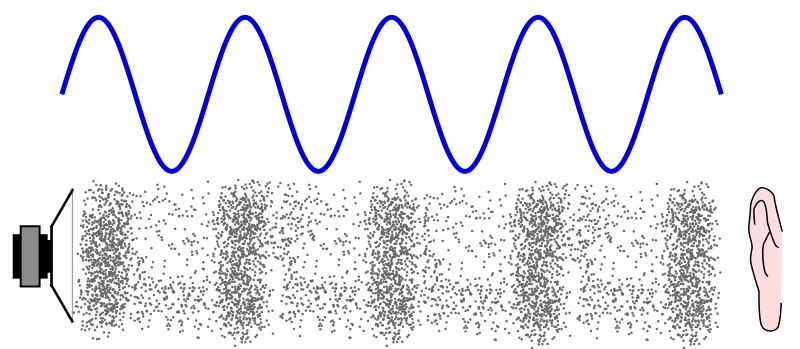
Sound is represented by such a waveform.

You can see a similar waveform even if you zoom in on the audio file in your DAW, but first let’s make this the waveform of the sound in the real world (analog world).

We take this to a computer and listen to it on a speaker and edit it, so we have to bring the sound as data into the digital world. (Convert DA)

At that point, a process called “sampling” is required, but this is not a particularly difficult story, and it is necessary to cut a cross section of sound tens of thousands of times per second and digitize analog data. .

And this “how many times per second do you sample?” it is expressed by the number “sampling rate”.

Old man
If the sample rate is 1 Hz, it means sample once per second.

So at 44.1kHz (44,100hz) CD sound quality, you’re sampling 44,100 times per second.

Next, let’s take a look at the waveform of sound reproduced in the digital world.

This part is the sampled part, and the more points there are, the more accurately the original sound can be reproduced.

In the figure above, the points are connected by a straight line, but a relatively smooth curve is still maintained at this point.

So what happens to the waveform if this point (sample rate) is low?

What is sample rate/sample frequency?

sample rate

Sampling rate Sampling rate is the number of sampling processes performed per second in an AD converter that converts an analog signal to a digital signal.

The unit is “Hz”, and the higher the value, the faster the analog input signal can be converted to a digital value, resulting in higher sound quality. However, the amount of data grows proportionally, so choose the right frequency for media and devices with limited storage capacity.

It is said that in order to accurately record and reproduce a certain sound, it is necessary to sample at a frequency that is approximately twice the frequency of that sound. The sample rate used on music CDs is 44.1 kHz. In this case, the voice waveform is shredded 44,100 times per second, and the voice information at each time is converted into digital information.

Human beings generally have 20 Hz for individual differences, but they can perceive sounds from around 15 kHz to 20 kHz as sound, and this frequency band is called the audible range.

Difference Between Sample Rate and Bit Rate
Sample rate and bit rate are used to describe the sound quality before and after the compression of the audio data.

The sampling rate is a value that represents “the number of sampling processes performed per second”.
For example, at the standard sample rate of 44.1 kHz, that means sampling 44,100 times per second.
The higher this number, the smoother the sound and the better the sound quality. In other words, the numerical value of the sample rate represents the quality of the sound.

On the other hand, the bitrate is a value that indicates “at how many levels the volume is rendered”.
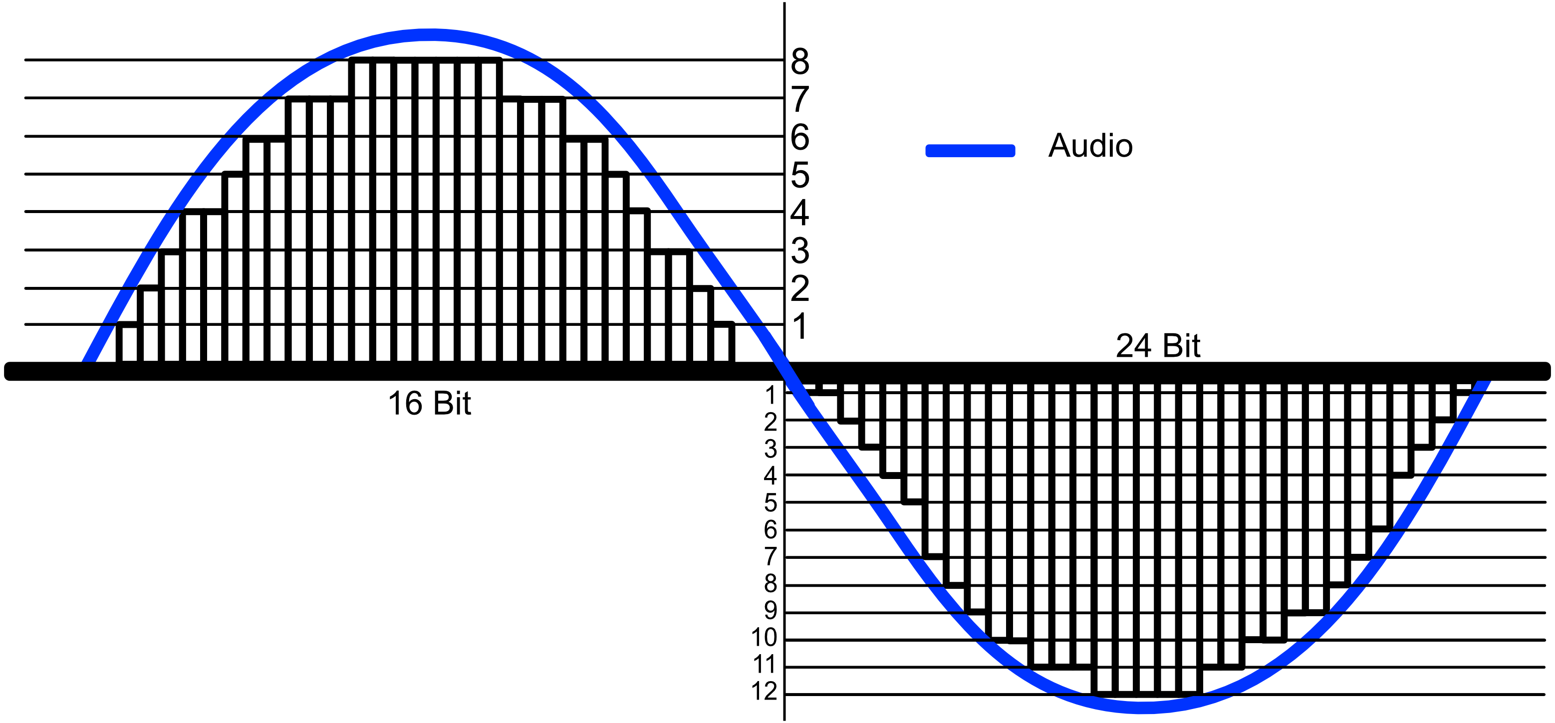
For example, in the case of 16 bits, which is the standard bit rate, the amount of information is divided by 2 to the 16th power (= 65536 steps). If the number of bits is low, the sound quality will be uneven, and as with the sample rate, the higher the bit rate value, the more information can be reproduced and the sound quality will be better.

The sample rate: looking for the best sound

When it comes to digital music and sound effects, the sample rate plays an important role. This applies to both CDs and file formats like MP3 and network players. The values specified for the height or frequency of the removal rate differ significantly from each other. An important reference value is 44.1 kHz. We explain why this is so.

Sample rate

What is sampling frequency about

For a guitar voice or riff to be stored on a CD or hard drive, the sound must be digitized. To do this, samples of the analog signal are taken at constant time intervals (discrete time). These are used to convert the recorded information into a code.

If the signal is digital, such as MP3, it can also be converted back to an analog signal, such as fluctuating current intensity, to make the membrane of a speaker sound. The frequency of these samples or samples is indicated by the sampling frequency. In general, the more samples there are, the more detailed the sound can be digitally reproduced.

A CD accepts signals that have been digitized with a sampling frequency of 44,100 Hz or 44.1 kHz. That corresponds to 44,100 samples per second. Of course, this frequency was not determined by chance. Such a resolution takes into account the maximum audible audio frequency of about 20 kHz and an important rule of data processing: the Nyquist-Shannon theorem. From this it can be deduced that the sampling frequency must be at least twice as high as the highest frequency of the signal to be digitized. So if the highest tones we can hear vibrate at 20 kHz, according to this theorem, the sample rate must be at least 40 kHz in order to digitize and decode all the tones correctly. Otherwise, the digitized signal can only be incorrectly converted to analog.

44.1 kHz is not the end of the story

The sampling frequency development did not stop at 44.1 kHz. Modern data carriers and transmission methods now make it possible to process significantly larger amounts of data. Lossless formats like FLAC or high resolution multi-channel standards exceed this value many times over.

Dolby TrueHD, for example, supports very high sample rates. Thus, significantly finer digitized signals can be processed. Additionally, audio masters can use better reconstruction and anti-aliasing filters.

Sample rate isn’t the only measure – bit depth

While the sample rate describes the frequency of the samples, the bit depth indicates how many bits are used per sample. In other words, the bit depth tells you how accurate or how high the resolution is for each individual sample. The amplitude or dynamic range of the analog signal at the time of the sample is determined. So the area between the weakest and strongest sound pressure level. On a CD, each sample is 16-bit deep, although this value is also exceeded by modern digital standards. Dolby TrueHD reaches 24 bits.

The Raumfeld connector brings out what is digitally possible
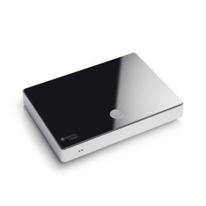
The raumfeld connector supports a sampling rate of 192 kHz.

▶ Hardly anyone makes bits sound as good as the Raumfeld plug. Because it plays high-resolution formats up to 96 kHz and 24-bit. An integrated high-end converter from Cirrus Logic converts digital data into analog. The Raumfeld connector has a powerful WLAN module for wireless data transmission. Thanks to Google Cast, multi-room speakers can also be conveniently controlled via the connector. If you connect the network player to a conventional system via Cinch or Toslink, it will be integrated into the local network.

Conclusion: sample rate as a bargaining chip for digital sound formats
The sampling rate indicates how often signals are sampled from an analog signal for digitization.
The Nyquist-Shannon theorem states that for the digitization to be true to the original, the sample rate must be at least twice the highest analog frequency.
CDs support sample rates up to 44.1 kHz. Modern formats, on the other hand, can reproduce 96 kHz and more.
Bit depth indicates how individual samples are resolved and influences the digitized dynamic range.
While CD samples have a 16-bit resolution, Dolby TrueHD, for example, reaches 24-bit.

Sample rate (Hz and kHz), resolution (bits), and bit rate (kBit / s) for music and audio

Because it always leads to misunderstandings, today there is a short explanation of the most important key figures for music and audio files. These basically apply to all uncompressed formats (WAV and AIFF). I’ll also go into the bitrate of compressed formats like MP3, WMV, and OGG below.

Sample Rates

Basic knowledge: An audio file stores a number at very short intervals that represents the level of the audio signal. During playback, the contour is calculated from this sequence of numbers.

Audio Sample Rate

An audio file can have multiple channels. Mono (one channel), stereo (2 channels), and 5.1 and 7.1 (Surround) are common. Each channel provides the information from one of the speakers and is a separate audio signal. That means we can split a stereo file and save it into two mono files.

The sample rate (Hertz) indicates how often the audio level is recorded and saved in one second. A specification of 44,100 Hz (44.1 kHz) means that 44,100 values are stored for one second of music. Typical sample rates are 44.1 kHz (music CD), 48.0 kHz (film), and 96 kHz (recording studio).

The resolution (bit) indicates how much memory is used for that sample value. For example, 16 bits (2 to the power of 16) allow a scale of 65,536 values for each individual sample value. If we have a lot of memory for a value, we can process the signal more precisely. Typical settings are 16-bit (music CD) or 24-bit or 32-bit in the studio.

Bit rate (kBit / s) is often confused with resolution. Represents the “bandwidth” of the audio file, that is, the amount of data that is processed in one second. For uncompressed formats like WAV and AIFF, you can easily calculate the bit rate by multiplying the above three values:

Bit rate = channels x sample rate x resolution

Example:

A WAV file in CD quality has the following bit rate:
2 channels x 16 bits x 44.1 kHz = 1411.2 kBit / s

The bit rate for compressed formats (MP3, OGG, WMV, AAC, etc.)
Unfortunately, this formula does not work with MP3 and other compressed formats because the signal is packaged to save space. The encoder reduces the bandwidth of the data to a desired bit rate and tries to obtain the best possible quality within this frame. The bit rate can be constant (CBR mode) or variable (VBR mode). A variable bit rate often makes sense if the audio signal is highly varied (for example, a movie or radio playback).

Sample rate, a clear explanation about what the sample rate is

Let’s proceed in order and start from the sampling frequency, defined as the number of times per second in which our AD converter will measure the electrical signal placed at its input: it is measured in Herz (Hz).

Obviously, the greater the number of “photographs” that we take of our electrical signal in one second, the greater its fidelity to the “original” sound wave. At the same time, obviously, our converter will be obliged to spend a greater amount of “energy” (faster information processing speed, greater storage space, etc.) which therefore translates into a different quality of components and obviously at a higher cost.

La tasa de muestreo

Sampling rate

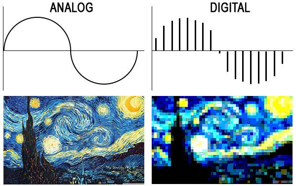
On the left an analog wave (a sine wave) in the time / amplitude domain and an image of Vincent Van Gogh’s “Starry Night” which, for our teaching purposes, we intend to be very high resolution. On the right, a quick reconstruction of the same sampled analog waveform and the same photograph reproduced with a much smaller number of pixels.

Well, if it were that simple, there wouldn’t be a bit of fun. Let’s go back to the diagram of the AD converter at the end of the previous article. Surely you have noticed that the first block through which our signal passes is the so-called “Anti-aliasing filter”, nothing less than a low pass filter.

Coooooooooooosaaaaaaaaaaaaaaaaaa !? Do we want to faithfully reproduce our signal in the digital domain and the first thing we do is pass it through a filter to change its frequency component (remove all components above a certain frequency)?

Yes my dear … you need to share a minimum (but I swear, a minimum) of signal theory to tell you a bit about the “Nyquist-Shannon Sampling Theorem” (for the “fetishists” – no offense, for course …. I am also part of it: of the mathematical treatment, take a look at the related Wikipedia page where you can find a good perspective), based on which, to sample an analog signal without loss of information (that is, to be able to re-enter it – then convert it DA – into the analog domain without “noticeable” differences compared to the original signal) it is necessary that the number of samples taken per second (the sampling frequency) is at least twice the maximum present frequency into the signal to be sampled, Therefore, it is worth introducing frequencies in the digital signal that do not exist in the original analog signal (the calls, and hence the filter name, alias frequencies).
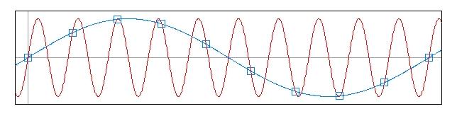
The aliasing phenomenon occurs because we do not have enough samples to describe the trend of the higher frequencies, which are therefore translated into the digital signal as lower frequencies, although nonexistent in the original signal. See this beautiful image always taken from the omniscient Wikipedia. In red the sinusoid sampled at intervals not sufficient to reconstruct it, and in blue the frequency alias (lower) that originates from the points we have taken.

La tasa de muestreo

Sampling rate

As we already know, the human ear is sensitive, at most (at an early age and in good hearing health), to frequencies around 20 KHz; In theory, our anti-aliasing filter should be set at 40,000 Hz and that should be our sample rate, but since it is practically impossible to build a filter with such a steep slope in analog, we opted for a filter with less steep slope and so both leaves the signal to sample frequencies slightly higher than 20,000 Hz (which we don’t hear, but there are), sampling at a slightly higher frequency. Therefore, the minimum sample rate used is equal to 44,100 samples per second.

Obviously, technological development and, nevertheless, the opinion and experience of many professionals (which I personally share very modestly) have in any case led to the awareness that, having set the minimum limit of 44,100 Hz (we will see later, it is the sampling frequency of the files that make up an audio CD), sampling at higher frequencies certainly leads to better results both from the point of view of signal manipulation (passing through a plug-in, the sum of two or more signals within a DAW, etc.) and from a listening point of view.

Later we will return to the topic, we will develop it further and we will begin to understand the logic with which the converter assigns a value in “machine language” to the different samples taken during the sampling phase.